badMIXTURE
jhmarcus
2019-04-16
Last updated: 2019-04-26
Checks: 5 1
Knit directory: drift-workflow/analysis/
This reproducible R Markdown analysis was created with workflowr (version 1.2.0). The Report tab describes the reproducibility checks that were applied when the results were created. The Past versions tab lists the development history.
The R Markdown file has unstaged changes. To know which version of the R Markdown file created these results, you’ll want to first commit it to the Git repo. If you’re still working on the analysis, you can ignore this warning. When you’re finished, you can run wflow_publish to commit the R Markdown file and build the HTML.
Great job! The global environment was empty. Objects defined in the global environment can affect the analysis in your R Markdown file in unknown ways. For reproduciblity it’s best to always run the code in an empty environment.
The command set.seed(20190211) was run prior to running the code in the R Markdown file. Setting a seed ensures that any results that rely on randomness, e.g. subsampling or permutations, are reproducible.
Great job! Recording the operating system, R version, and package versions is critical for reproducibility.
Nice! There were no cached chunks for this analysis, so you can be confident that you successfully produced the results during this run.
Great! You are using Git for version control. Tracking code development and connecting the code version to the results is critical for reproducibility. The version displayed above was the version of the Git repository at the time these results were generated.
Note that you need to be careful to ensure that all relevant files for the analysis have been committed to Git prior to generating the results (you can use wflow_publish or wflow_git_commit). workflowr only checks the R Markdown file, but you know if there are other scripts or data files that it depends on. Below is the status of the Git repository when the results were generated:
Ignored files:
    Ignored:    .Rhistory
    Ignored:    analysis/.Rhistory
    Ignored:    analysis/figure/
    Ignored:    analysis/flash_cache/
    Ignored:    data.tar.gz
    Ignored:    data/datasets/
    Ignored:    data/raw/
    Ignored:    output.tar.gz
    Ignored:    output/

Unstaged changes:
    Modified:   analysis/badmixture.Rmd
    Modified:   analysis/simple_tree_simulation.Rmd
    Modified:   code/viz.R
Note that any generated files, e.g. HTML, png, CSS, etc., are not included in this status report because it is ok for generated content to have uncommitted changes.
These are the previous versions of the R Markdown and HTML files. If you’ve configured a remote Git repository (see ?wflow_git_remote), click on the hyperlinks in the table below to view them.
| File | Version | Author | Date | Message |
|---|---|---|---|---|
| Rmd | e33ede5 | jhmarcus | 2019-04-24 | updated pop names in badmixture |
| html | e33ede5 | jhmarcus | 2019-04-24 | updated pop names in badmixture |
| Rmd | e32adcc | jhmarcus | 2019-04-19 | init badmixture sim |
| html | e32adcc | jhmarcus | 2019-04-19 | init badmixture sim |
| Rmd | 1a21d43 | jhmarcus | 2019-04-17 | updated simple tree doc |
Here I perform simulations from Lawson et al. 2018. These simulations are specifically designed to illustrate challenges with interpreting admixture coefficients from PSD models as population genetic parameters. Specifically they ran ADMIXTURE (K=11) on three challenging simulation scenarios which are inspired by human demographic histories. They find ADMIXTURE generates the same coefficients under these three different scenarios. The figure below and found in the supplement of the badMIXTURE paper visually describes the simulation settings:

Here I attempt to replicate their findings by running ADMIXTURE on the same datasets simulated in the paper as well as running FLASH (Drift) to see if it can distinguish these models. Note, I downloaded the plink files from their simulations from here. I then filtered on any missingness and removed variants with minor allele frequency less than 5%.
Imports
Lets import some needed packages:
library(ggplot2)
library(tidyr)
library(dplyr)
library(RColorBrewer)
library(knitr)
source("../code/viz.R")
source("../code/prep.R")
Data
It took some communication with the authors of badMIXTURE to hunt this information down i.e. how the population ids in the plink file map to the supplementary figure 1 from the badMIXTURE paper. Note that Pop10 / MidE1 is simulated but not sampled in the plink files.
pops_old = c("Pop1", "Pop2", "Pop3", "Pop4",
             "Pop7", "Pop5", "Pop6", "Pop13",
             "Pop8", "Pop9", "Pop11", "Pop12")
pops = c("Afr1", "Afr2", "Afr3", "Afr4",
         "P1", "P2", "P3", "P4",
         "Eur1", "Eur2", "EA1", "EA2")
pop_df = data.frame(pop_o=pops_old, pop=pops)
pops4 = paste0("P", 1:4)
pop_df %>% head()
pop_o pop
1 Pop1 Afr1
2 Pop2 Afr2
3 Pop3 Afr3
4 Pop4 Afr4
5 Pop7 P1
6 Pop5 P2ADMIXTURE
Here the colors of the factors between the three ADMIXTURE runs changes (I need to work on factor color matching code) but one can see the similarities in the highlighted 4 populations.
Recent (Recent Admixture)
l_df = read.table("../output/admixture/recent_sim/Recent_admix_geno_maf.K11r1.Q", sep=" ", header=F)
K = ncol(l_df)
colnames(l_df) = 1:K
inds = read.table("../data/datasets/recent_sim/Recent_admix_geno_maf.fam", header=F, stringsAsFactors=F) %>% pull(V2)
pops = read.table("../data/datasets/recent_sim/Recent_admix_geno_maf.fam", header=F, stringsAsFactors=F) %>% pull(V1)
l_df$ID = inds
l_df$pop_o = pops

l_df = l_df %>% inner_join(pop_df, on="pop_o") %>% select(-pop_o)
Joining, by = "pop_o"Warning: Column `pop_o` joining character vector and factor, coercing into
character vectorl_df$ID = factor(l_df$ID, levels = l_df$ID) # make sure the ids are sorted
l_gath_df = l_df %>% gather(K, value, -ID, -pop)
l_gath_df4 = l_df %>% gather(K, value, -ID, -pop) %>% filter(pop %in% pops4)
pall = structure_plot(gath_df=l_gath_df, colset="Set3", facet_levels=pop_df$pop,
facet_grp="pop", label_size=5, fact_type="structure") +
theme(plot.title = element_text(size=6))
p4 = structure_plot(gath_df=l_gath_df4, colset="Set3", facet_levels=pops4,
facet_grp="pop", label_size=5, fact_type="structure") +
theme(plot.title = element_text(size=6))
p = cowplot::plot_grid(pall, p4, nrow = 2, align = "v") Warning in align_plots(plotlist = plots, align = align, axis = axis):
Complex graphs cannot be vertically aligned unless axis parameter is set
properly. Placing graphs unaligned.print(p)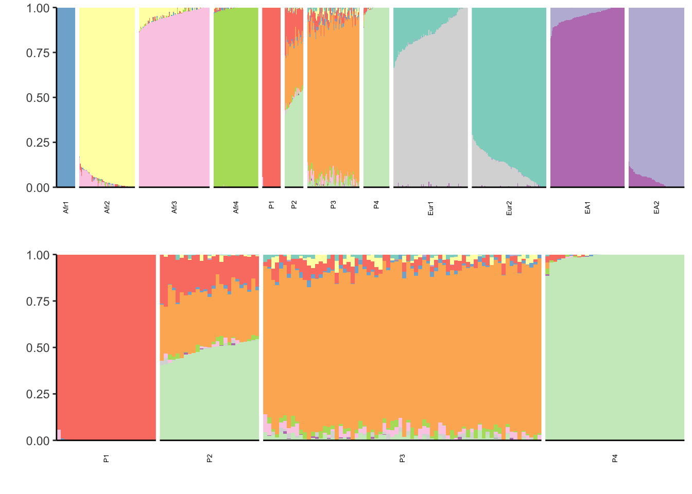
The data here sees to be pretty clustered for instance essentially a single factor explains Afr1, Afr4, P1, P4. Thus there is no why to really discern the hierarchical nature of the data.
Marginalisation (Recent Bottleneck)
l_df = read.table("../output/admixture/marginalisation_sim/Marginalisation_admix_geno_maf.K11r1.Q", sep=" ", header=F)
K = ncol(l_df)
colnames(l_df) = 1:K
inds = read.table("../data/datasets/marginalisation_sim/Marginalisation_admix_geno_maf.fam", header=F, stringsAsFactors=F) %>% pull(V1)
pops = read.table("../data/datasets/marginalisation_sim/Marginalisation_admix_geno_maf.fam", header=F, stringsAsFactors=F) %>% pull(V2)
l_df$ID = inds
l_df$pop_o = pops

l_df = l_df %>% inner_join(pop_df, on="pop_o") %>% select(-pop_o)
Joining, by = "pop_o"Warning: Column `pop_o` joining character vector and factor, coercing into
character vectorl_df$ID = factor(l_df$ID, levels = l_df$ID) # make sure the ids are sorted
l_gath_df = l_df %>% gather(K, value, -ID, -pop)
l_gath_df4 = l_df %>% gather(K, value, -ID, -pop) %>% filter(pop %in% pops4)
pall = structure_plot(gath_df=l_gath_df, colset="Set3", facet_levels=pop_df$pop,
facet_grp="pop", label_size=5, fact_type="structure") +
theme(plot.title = element_text(size=6))
p4 = structure_plot(gath_df=l_gath_df4, colset="Set3", facet_levels=pops4,
facet_grp="pop", label_size=5, fact_type="structure") +
theme(plot.title = element_text(size=6))
p = cowplot::plot_grid(pall, p4, nrow = 2, align = "v") Warning in align_plots(plotlist = plots, align = align, axis = axis):
Complex graphs cannot be vertically aligned unless axis parameter is set
properly. Placing graphs unaligned.print(p)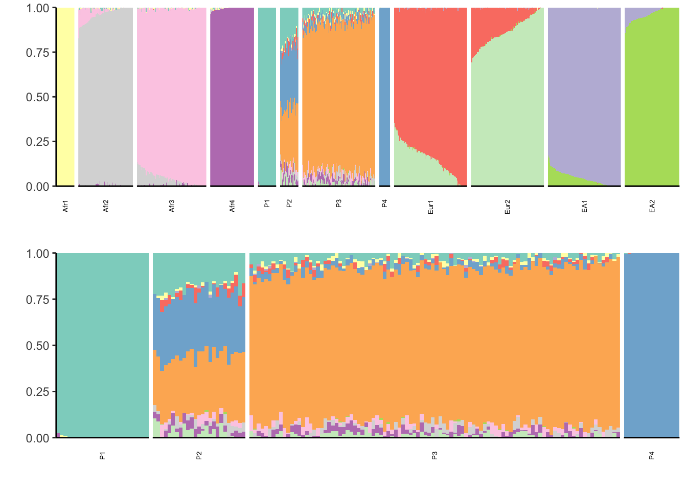
Interestingly the results look essentially the same (but with different colors). In some sense its good that the results are the same for the pops not P1-P4 but its troubling we generate the same admixture proportions under a different model.
Remnants (Ghost Admixture)
There is something very funky about the Remnants simulation. See populations 8-13.
l_df = read.table("../output/admixture/remnants_sim/Remnants_admix_geno_maf.K11r1.Q", sep=" ", header=F)
K = ncol(l_df)
colnames(l_df) = 1:K
inds = read.table("../data/datasets/remnants_sim/Remnants_admix_geno_maf.fam", header=F, stringsAsFactors=F) %>% pull(V1)
pops = read.table("../data/datasets/remnants_sim/Remnants_admix_geno_maf.fam", header=F, stringsAsFactors=F) %>% pull(V2)
l_df$ID = inds
l_df$pop_o = pops
l_df = l_df %>% inner_join(pop_df, on="pop_o") %>% select(-pop_o)
Joining, by = "pop_o"Warning: Column `pop_o` joining character vector and factor, coercing into
character vectorl_df$ID = factor(l_df$ID, levels = l_df$ID) # make sure the ids are sorted
l_gath_df = l_df %>% gather(K, value, -ID, -pop)
l_gath_df4 = l_df %>% gather(K, value, -ID, -pop) %>% filter(pop %in% pops4)
pall = structure_plot(gath_df=l_gath_df, colset="Set3", facet_levels=pop_df$pop,
facet_grp="pop", label_size=5, fact_type="structure") +
theme(plot.title = element_text(size=6))
p4 = structure_plot(gath_df=l_gath_df4, colset="Set3", facet_levels=pops4,
facet_grp="pop", label_size=5, fact_type="structure") +
theme(plot.title = element_text(size=6))
p = cowplot::plot_grid(pall, p4, nrow = 2, align = "v") Warning in align_plots(plotlist = plots, align = align, axis = axis):
Complex graphs cannot be vertically aligned unless axis parameter is set
properly. Placing graphs unaligned.print(p)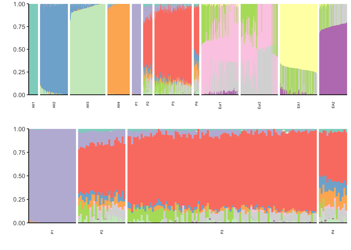
There is something wrong with this simulation … I need to follow up with the authors b/c this is way nosier then I expected.
FLASH-Greedy
Recent (Recent Admixture)
flash_fit = readRDS("../output/flash_greedy/recent_sim/Recent_admix_geno_maf.rds")
plot_pve(flash_fit)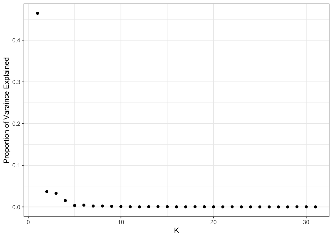
print(flash_fit$pve) [1] 4.644314e-01 3.672962e-02 3.293419e-02 1.533617e-02 3.460167e-03
[6] 4.380101e-03 2.193011e-03 2.220532e-03 1.516786e-03 7.452720e-04
[11] 3.638727e-04 2.204384e-04 4.979738e-04 5.088945e-04 5.083526e-04
[16] 2.872698e-04 2.060834e-04 3.908611e-04 3.955174e-04 2.987267e-04
[21] 1.552774e-04 2.467179e-04 1.647525e-04 1.561975e-04 9.676400e-05
[26] 8.065071e-05 1.010647e-04 7.148456e-05 2.887337e-04 2.635893e-04
[31] 1.846785e-04It looks like the pve drops off at around 10 factors so lets go with visualizing the top 10:
l_df = as.data.frame(flash_fit$loadings$normalized.loadings[[1]])
colnames(l_df)[1:31] = 1:31
inds = read.table("../data/datasets/recent_sim/Recent_admix_geno_maf.fam", header=F, stringsAsFactors=F) %>%
       pull(V2)
pops = read.table("../data/datasets/recent_sim/Recent_admix_geno_maf.fam", header=F, stringsAsFactors=F) %>%
       pull(V1)
l_df$ID = inds
l_df$pop_o = pops
l_df = l_df %>% inner_join(pop_df, on="pop_o") %>% select(-pop_o)
Joining, by = "pop_o"Warning: Column `pop_o` joining character vector and factor, coercing into
character vectorfactors_incl = paste0(2:10)
l_gath_df = l_df %>%
select_if(~sum(!is.na(.)) > 0) %>%
gather(K, value, -ID, -pop) %>%
filter(K %in% factors_incl)
l_gath_df4 = l_df %>%
filter(pop %in% pops4) %>%
select_if(~sum(!is.na(.)) > 0) %>%
gather(K, value, -ID, -pop) %>%
filter(K %in% factors_incl)
pall = structure_plot(gath_df=l_gath_df, colset="Set3", facet_levels=pop_df$pop,
facet_grp="pop", label_size=5, fact_type="nonnegative") +
theme(plot.title = element_text(size=6))
p4 = structure_plot(gath_df=l_gath_df4, colset="Set3", facet_levels=pops4,
facet_grp="pop", label_size=5, keep_leg=TRUE,
fact_type="nonnegative") +
theme(plot.title = element_text(size=6))
p = cowplot::plot_grid(pall, p4, nrow = 2)
print(p)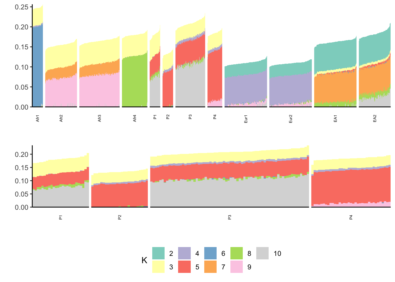
Looks pretty clean! It is much easier to observe some hierarchical structure to the data i.e. the purple factor is in all African populations, the yellow factor is in out of Africa populations, the green factor is only in East Asian populations, the red factor is only in European populations, and then there are population / sub-population specific-ish factors i.e. pink, orange, gray. The ability to extract this type of hierarchical structure is incredibly cool. I need to think more about how “recent admixture” is represented in P1-P4.
Marginalisation (Recent Bottleneck)
flash_fit = readRDS("../output/flash_greedy/marginalisation_sim/Marginalisation_admix_geno_maf.rds")
plot_pve(flash_fit)
print(flash_fit$pve) [1] 4.650849e-01 3.675585e-02 3.233046e-02 1.511297e-02 4.308358e-03
[6] 2.896828e-03 2.464024e-03 2.282352e-03 6.153068e-04 5.829713e-04
[11] 4.275390e-04 5.578858e-04 5.114740e-04 3.479125e-04 1.310698e-04
[16] 6.477571e-04 3.644369e-04 8.658475e-05 2.993560e-04 4.205884e-04
[21] 4.013920e-04 2.405113e-04 1.489529e-04 3.378401e-04 1.160602e-04
[26] 2.484946e-04 1.684698e-04 1.800022e-04 2.718841e-04 1.748917e-04
[31] 2.117316e-04This also seems to drop off at 10 factors so lets visualize that:
l_df = as.data.frame(flash_fit$loadings$normalized.loadings[[1]])
colnames(l_df)[1:31] = 1:31
inds = read.table("../data/datasets/marginalisation_sim/Marginalisation_admix_geno_maf.fam", header=F, stringsAsFactors=F) %>% pull(V1)
pops = read.table("../data/datasets/marginalisation_sim/Marginalisation_admix_geno_maf.fam", header=F, stringsAsFactors=F) %>% pull(V2)
l_df$ID = inds
l_df$pop_o = pops
l_df = l_df %>% inner_join(pop_df, on="pop_o") %>% select(-pop_o)
Joining, by = "pop_o"Warning: Column `pop_o` joining character vector and factor, coercing into
character vectorfactors_incl = paste0(2:10)
l_gath_df = l_df %>%
select_if(~sum(!is.na(.)) > 0) %>%
gather(K, value, -ID, -pop) %>%
filter(K %in% factors_incl)
l_gath_df4 = l_df %>%
filter(pop %in% pops4) %>%
select_if(~sum(!is.na(.)) > 0) %>%
gather(K, value, -ID, -pop) %>%
filter(K %in% factors_incl)
pall = structure_plot(gath_df=l_gath_df, colset="Set3", facet_levels=pop_df$pop,
facet_grp="pop", label_size=5, fact_type="nonnegative") +
theme(plot.title = element_text(size=6))
p4 = structure_plot(gath_df=l_gath_df4, colset="Set3", facet_levels=pops4,
facet_grp="pop", label_size=5, keep_leg=TRUE, fact_type="nonnegative") +
theme(plot.title = element_text(size=6))
p = cowplot::plot_grid(pall, p4, nrow = 2)
print(p)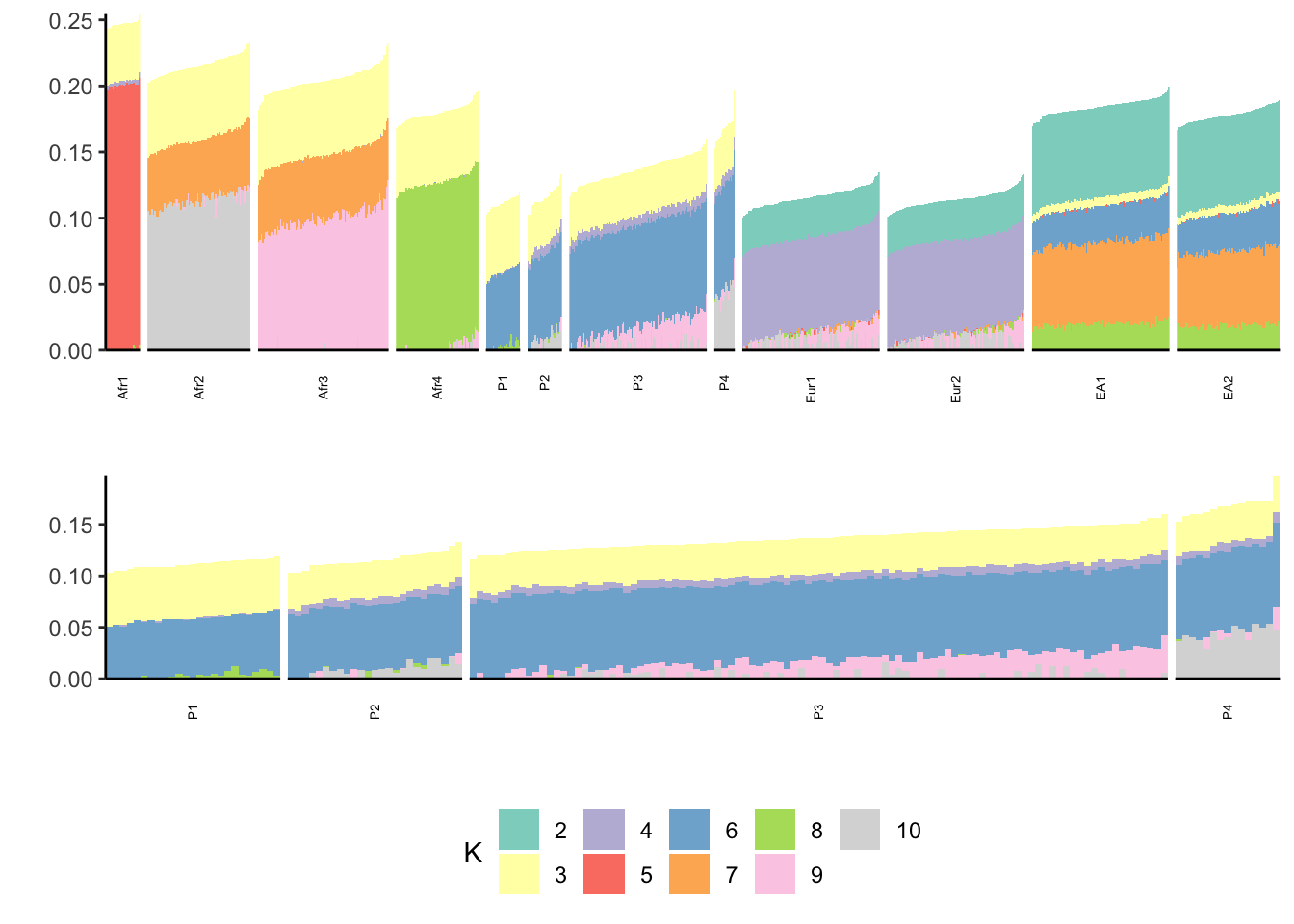
There are a lot of similarities to the past results but there are differences as well! I need to think more about how P1-P4 reflect a recent bottleneck.
Remnants (Ghost Admixture)
flash_fit = readRDS("../output/flash_greedy/remnants_sim/Remnants_admix_geno_maf.rds")
plot_pve(flash_fit)
print(flash_fit$pve) [1] 4.650896e-01 3.224806e-02 3.719610e-02 1.446442e-02 3.490551e-03
[6] 2.377310e-03 1.795288e-03 2.196230e-03 2.981648e-03 8.615182e-04
[11] 5.692530e-04 4.063218e-04 5.629490e-04 2.410158e-04 2.481862e-04
[16] 4.541307e-04 2.923784e-04 3.260667e-04 2.663500e-04 6.961251e-05
[21] 3.122211e-04 2.113871e-04 2.954215e-04 3.431343e-04 7.240811e-05
[26] 1.982314e-04 1.477614e-04 1.569933e-04 7.707317e-05 8.636696e-05
[31] 1.029189e-04Yet again seems to drop off at 10 factors:
l_df = as.data.frame(flash_fit$loadings$normalized.loadings[[1]])
colnames(l_df)[1:31] = 1:31
inds = read.table("../data/datasets/remnants_sim/Remnants_admix_geno_maf.fam", header=F, stringsAsFactors=F) %>% pull(V1)
pops = read.table("../data/datasets/remnants_sim/Remnants_admix_geno_maf.fam", header=F, stringsAsFactors=F) %>% pull(V2)
l_df$ID = inds
l_df$pop_o = pops
l_df = l_df %>% inner_join(pop_df, on="pop_o") %>% select(-pop_o)
Joining, by = "pop_o"Warning: Column `pop_o` joining character vector and factor, coercing into
character vectorfactors_incl = paste0(2:10)
l_gath_df = l_df %>%
select_if(~sum(!is.na(.)) > 0) %>%
gather(K, value, -ID, -pop) %>%
filter(K %in% factors_incl)
l_gath_df4 = l_df %>%
filter(pop %in% pops4) %>%
select_if(~sum(!is.na(.)) > 0) %>%
gather(K, value, -ID, -pop) %>%
filter(K %in% factors_incl)
pall = structure_plot(gath_df=l_gath_df, colset="Set3", facet_levels=pop_df$pop,
facet_grp="pop", label_size=5, fact_type="nonnegative") +
theme(plot.title = element_text(size=6))
p4 = structure_plot(gath_df=l_gath_df4, colset="Set3", facet_levels=pops4,
facet_grp="pop", label_size=5, keep_leg=TRUE, fact_type="nonnegative") +
theme(plot.title = element_text(size=6))
p = cowplot::plot_grid(pall, p4, nrow = 2)
print(p)
| Version | Author | Date |
|---|---|---|
| e33ede5 | jhmarcus | 2019-04-24 |
ADMIXTURE results looked really funky as well.
sessionInfo()R version 3.5.1 (2018-07-02)
Platform: x86_64-apple-darwin13.4.0 (64-bit)
Running under: macOS 10.14.2
Matrix products: default
BLAS/LAPACK: /Users/jhmarcus/miniconda3/lib/R/lib/libRblas.dylib
locale:
[1] en_US.UTF-8/en_US.UTF-8/en_US.UTF-8/C/en_US.UTF-8/en_US.UTF-8
attached base packages:
[1] stats graphics grDevices utils datasets methods base
other attached packages:
[1] knitr_1.21 RColorBrewer_1.1-2 dplyr_0.8.0.1
[4] tidyr_0.8.2 ggplot2_3.1.0
loaded via a namespace (and not attached):
[1] Rcpp_1.0.0 compiler_3.5.1 pillar_1.3.1 git2r_0.23.0
[5] plyr_1.8.4 workflowr_1.2.0 tools_3.5.1 digest_0.6.18
[9] evaluate_0.12 tibble_2.0.1 gtable_0.2.0 pkgconfig_2.0.2
[13] rlang_0.3.1 yaml_2.2.0 xfun_0.4 flashier_0.1.1
[17] withr_2.1.2 stringr_1.4.0 fs_1.2.6 rprojroot_1.3-2
[21] grid_3.5.1 tidyselect_0.2.5 cowplot_0.9.4 glue_1.3.0
[25] R6_2.4.0 rmarkdown_1.11 reshape2_1.4.3 purrr_0.3.0
[29] magrittr_1.5 whisker_0.3-2 backports_1.1.3 scales_1.0.0
[33] htmltools_0.3.6 assertthat_0.2.0 colorspace_1.4-0 labeling_0.3
[37] stringi_1.2.4 lazyeval_0.2.1 munsell_0.5.0 crayon_1.3.4