Fitting a real-data covariance matrix: interpretation

Superpopulations

covmat <- readRDS("../data/datasets/1kg_phase3_derived/1kg_phase3_derived_covmat.rds")
meta <- readRDS("../data/datasets/1kg_phase3_derived/1kg_phase3_derived_meta.rds")

plot_fl <- function(LL) {
  df <- data.frame(LL)
  colnames(df) <- paste0("Factor ", formatC(1:ncol(LL), width = 2, flag = "0"))
  df$subpop <- meta$pop
  df$superpop <- meta$super_pop
  df <- df %>% arrange(superpop, subpop)
  df$idx <- 1:nrow(df)
  gath_df <- df %>% 
    gather(K, value, -subpop, -idx, -superpop) %>%
    mutate(K = factor(K))
  med_gath_df <- gath_df %>% 
    group_by(subpop, K) %>% 
    summarise(value=median(value), idx=median(idx))
  
  p <- ggplot(gath_df, aes(x=idx, y=value, color=superpop)) + 
    geom_point() +
    facet_wrap(~K) + 
    geom_hline(yintercept = 0, linetype = "dashed") +
    theme(axis.title.x=element_blank(),
          axis.text.x=element_blank(),
          axis.ticks.x=element_blank()) +
    labs(color="superpop")
  return(p)
}

plot_subpops <- function(LL) {
  df <- data.frame(LL)
  colnames(df) <- paste0("Factor ", formatC(1:ncol(LL), width = 2, flag = "0"))
  df$subpop <- meta$pop
  df$superpop <- meta$super_pop
  df <- df %>% arrange(superpop, subpop)
  df$idx <- 1:nrow(df)
  gath_df <- df %>% 
    gather(K, value, -subpop, -idx, -superpop) %>%
    mutate(K = factor(K))
  med_gath_df <- gath_df %>% 
    group_by(subpop, K) %>% 
    summarise(value=median(value), idx=median(idx))
  
  all_plots <- lapply(levels(df$superpop), function(pop) {
    p <- ggplot(filter(gath_df, superpop == pop), aes(x=idx, y=value, color=subpop)) + 
      geom_point() +
      facet_wrap(~K) + 
      geom_hline(yintercept = 0, linetype = "dashed") +
      theme(axis.title.x=element_blank(),
            axis.text.x=element_blank(),
            axis.ticks.x=element_blank()) +
      labs(color="subpop") +
      ggtitle(paste("superpop:", pop))
    return(p)  
  })
}

t_greedy <- system.time({
  ones <- matrix(1, nrow = nrow(covmat), ncol = 1)
  ls.soln <- t(solve(crossprod(ones), crossprod(ones, covmat)))
  
  covmat_diagNA <- covmat
  diag(covmat_diagNA) <- NA
  
  fl_g <- flash.init(covmat_diagNA) %>%
    flash.set.verbose(0) %>%
    flash.init.factors(EF = list(ones, ls.soln)) %>%
    flash.fix.loadings(kset = 1, mode = 1) %>%
    flash.backfit() %>%
    flash.add.greedy(Kmax = 11, 
                     prior.family = prior.point.laplace())
})

cat("Time to fit greedy factors:", round(t_greedy[3], 1), "seconds")

#> Time to fit greedy factors: 41.9 seconds

t_backfit <- system.time({
  fl_bf <- fl_g %>% flash.backfit(maxiter = 1000)
})

cat("Time to backfit:", round(t_backfit[3] / 60, 1), "minutes")

#> Time to backfit: 35.7 minutes

LL <- fl_bf$loadings.pm[[1]] %*% diag(sqrt(fl_bf$loadings.scale))
LL <- LL[, c(1, rep(2:fl_bf$n.factors, each = 2))]
LL <- t(t(LL) * c(1, rep(c(1, -1), fl_bf$n.factors - 1)))
LL <- pmax(LL, 0)

LL_scale <- apply(LL, 2, max)
LL <- t(t(LL) / LL_scale)

t_drift <- system.time({
  dr <- init_from_covmat(covmat, LL, p = 10000, prior.s2 = LL_scale^2, fix.EL = 1,
                         prior.family = prior.bimodal())
  dr <- drift(dr, maxiter = 500, tol = 1e-4, verbose = FALSE)
})

cat("Time to drift:", round(t_drift[3] / 60, 1), "minutes")

#> Time to drift: 11.9 minutes

LL <- dr$EL %*% diag(sqrt(dr$prior_s2))
LL_norms <- apply(LL, 2, function(x) sum(x^2))
LL <- LL[, order(LL_norms, decreasing = TRUE)]
LL_norms <- apply(LL, 2, function(x) sum(x^2))
zero_cols <- which(LL_norms < 1e-6)
LL <- LL[, -zero_cols]

plot(plot_fl(LL))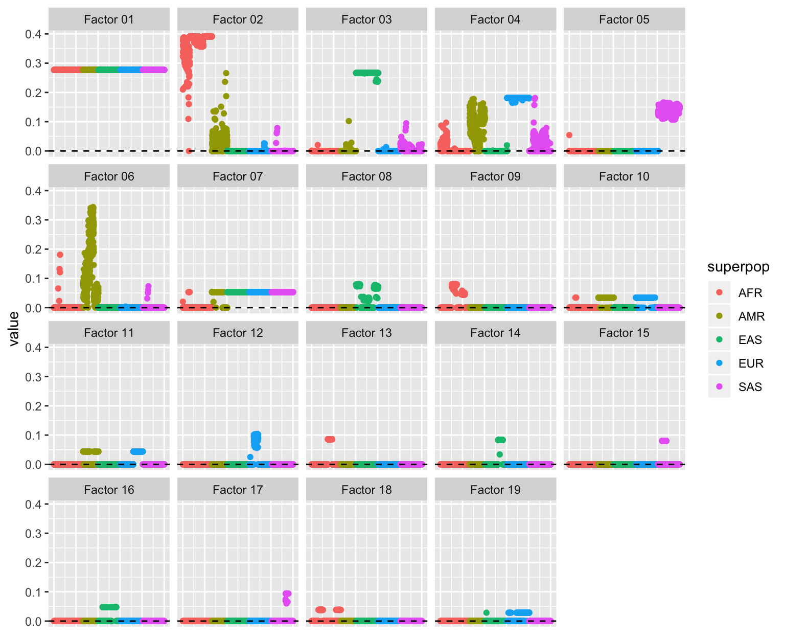

Subpopulations

all_p <- plot_subpops(LL)
for (p in all_p) {plot(p)}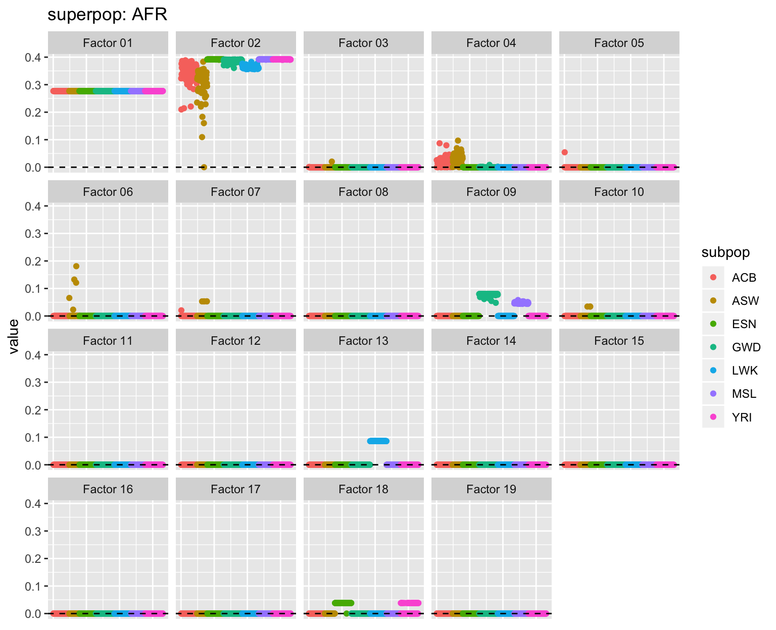

Factor descriptions

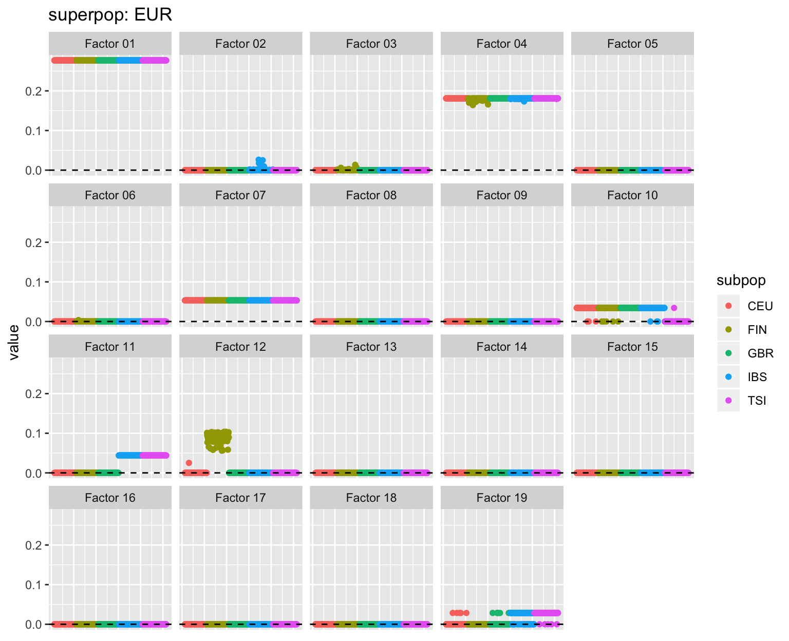
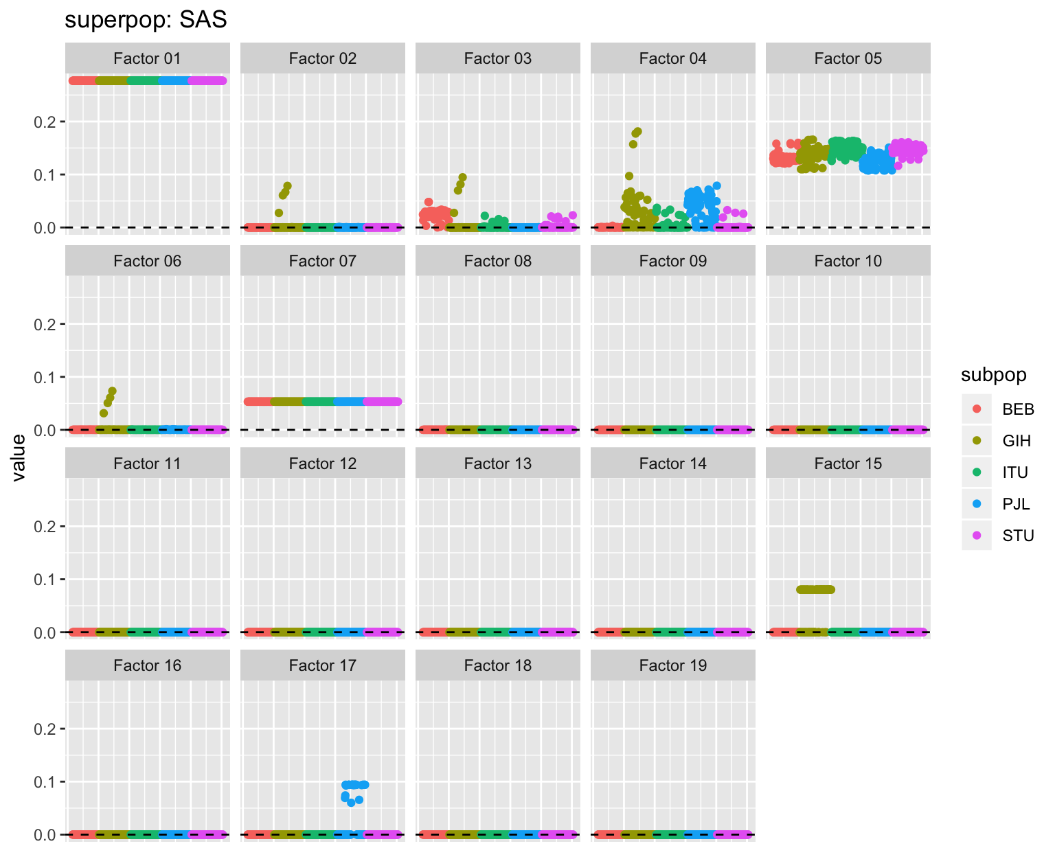
• Factor 2: The primary African factor, with varying degrees of admixture for African Americans (ASW), African Caribbeans (ACB), and Amerindians. Intriguingly, there is a small degree of admixture for several Iberians (IBR) and Gujarati Indians from Houston (GIH).

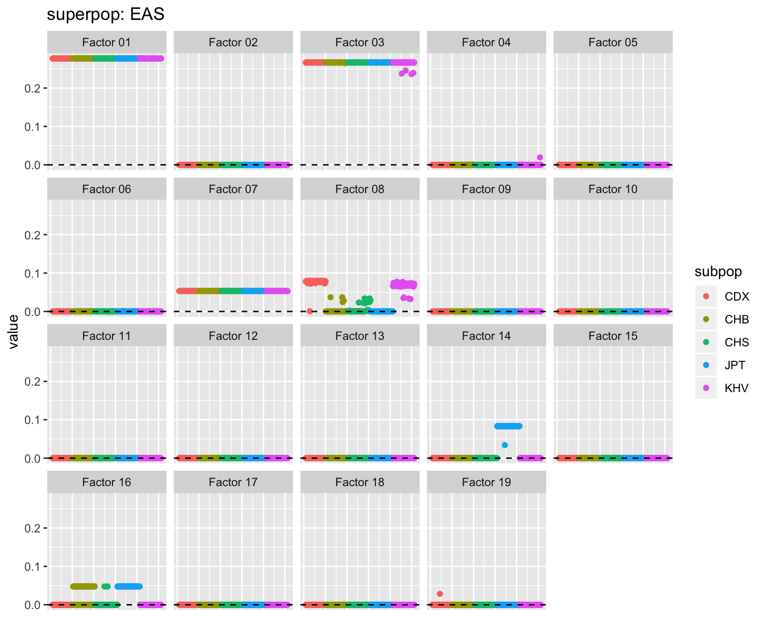
• Factor 3: The primary East Asian factor. There is a very small amount of admixture for Peruvians (PEL) as well as for a small number of African Americans, Mexicans (MXL), and Finns (FIN). A small degree of admixture is common among Bengali (BEB) and Telugu (ITU) Indians and Sri Lankans (STU), and present but less common among Gujarati Indians.

• Factor 4: The primary European factor, with strong contributions from South Asian populations (especially Punjabi and Gujarati) and varying degrees of admixture for African Americans, African Caribbeans, and Amerindians. There is a single Vietnamese (KHV) individual with a nonzero loading: this can probably be ignored.

• Factor 5: The primary South Asian factor. There is a single African Caribbean individual with a nonzero loading.

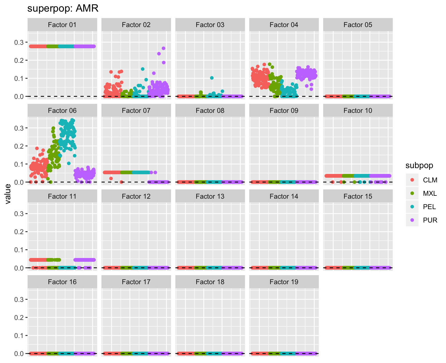
• Factor 6: The Amerindian factor, with loadings largest among Peruvians and smallest among Puerto Ricans (PUR). Several African Caribbeans are loaded on this factor, as well as, interestingly, a few Gujarati Indians from Houston.

• Factor 7: The out-of-Africa factor. Oddly, it is shared by Mexicans, Peruvians, and most Columbians (CLM), but not by most Puerto Ricans.

• Factor 8: Substructure among East Asians: large loadings for the more Southeastern Vietnamese and Chinese Dai populations, modest loadings for some Chinese Han, and mostly zero loadings for Japanese.

• Factor 9: A West African factor: large loadings for Gambians (GWD) and modest loadings for the Mende from Sierra Leone (MSL).

• Factor 10: Shared by all Amerindian and European populations except for Toscani. I don’t know where this comes from.

• Factor 11: A Mediterranean factor, possibly? Shared by Southern European (Iberian and Toscani) and Puerto Rican populations and a large number of Mexicans and Colombians.

• Factor 12: A Finnish factor, also present among one or two Utah residents with European ancestry (CEU).

• Factor 13: Kenyan.

• Factor 14: Japanese.

• Factor 15: Common to some, but not all Gujarati Indians from Houston.

• Factor 16: Shared among Japanese, most Chinese Han from Beijing, and some Southern Chinese Han.

• Factor 17: Common to some, but not all Punjabi.

• Factor 18: Shared among the two Nigerian populations (Esan (ESN) and Yoruba (YRI)).

• Factor 19: Shared among most Toscani and Iberians and some British and Utah residents. One Chinese Dai individual has a nonzero loading.
  
  

  Session information

sessionInfo()

#> R version 3.5.3 (2019-03-11)
#> Platform: x86_64-apple-darwin15.6.0 (64-bit)
#> Running under: macOS Mojave 10.14.6
#> 
#> Matrix products: default
#> BLAS: /Library/Frameworks/R.framework/Versions/3.5/Resources/lib/libRblas.0.dylib
#> LAPACK: /Library/Frameworks/R.framework/Versions/3.5/Resources/lib/libRlapack.dylib
#> 
#> locale:
#> [1] en_US.UTF-8/en_US.UTF-8/en_US.UTF-8/C/en_US.UTF-8/en_US.UTF-8
#> 
#> attached base packages:
#> [1] stats     graphics  grDevices utils     datasets  methods   base     
#> 
#> other attached packages:
#>  [1] forcats_0.4.0      stringr_1.4.0      dplyr_0.8.0.1     
#>  [4] purrr_0.3.2        readr_1.3.1        tidyr_0.8.3       
#>  [7] tibble_2.1.1       ggplot2_3.2.0      tidyverse_1.2.1   
#> [10] drift.alpha_0.0.11 flashier_0.2.7    
#> 
#> loaded via a namespace (and not attached):
#>  [1] Rcpp_1.0.4.6      lubridate_1.7.4   invgamma_1.1     
#>  [4] lattice_0.20-38   assertthat_0.2.1  rprojroot_1.3-2  
#>  [7] digest_0.6.18     truncnorm_1.0-8   R6_2.4.0         
#> [10] cellranger_1.1.0  plyr_1.8.4        backports_1.1.3  
#> [13] evaluate_0.13     httr_1.4.0        pillar_1.3.1     
#> [16] rlang_0.4.2       lazyeval_0.2.2    readxl_1.3.1     
#> [19] rstudioapi_0.10   ebnm_0.1-21       irlba_2.3.3      
#> [22] whisker_0.3-2     Matrix_1.2-15     rmarkdown_1.12   
#> [25] labeling_0.3      munsell_0.5.0     mixsqp_0.3-40    
#> [28] broom_0.5.1       compiler_3.5.3    modelr_0.1.5     
#> [31] xfun_0.6          pkgconfig_2.0.2   SQUAREM_2017.10-1
#> [34] htmltools_0.3.6   tidyselect_0.2.5  workflowr_1.2.0  
#> [37] withr_2.1.2       crayon_1.3.4      grid_3.5.3       
#> [40] nlme_3.1-137      jsonlite_1.6      gtable_0.3.0     
#> [43] git2r_0.25.2      magrittr_1.5      scales_1.0.0     
#> [46] cli_1.1.0         stringi_1.4.3     reshape2_1.4.3   
#> [49] fs_1.2.7          xml2_1.2.0        generics_0.0.2   
#> [52] tools_3.5.3       glue_1.3.1        hms_0.4.2        
#> [55] parallel_3.5.3    yaml_2.2.0        colorspace_1.4-1 
#> [58] ashr_2.2-51       rvest_0.3.4       knitr_1.22       
#> [61] haven_2.1.1