Empircal Bayes Normal Means with Bimodal Priors
jhmarcus
2019-05-05
Last updated: 2019-05-06
Checks: 5 1
Knit directory: drift-workflow/analysis/
This reproducible R Markdown analysis was created with workflowr (version 1.2.0). The Report tab describes the reproducibility checks that were applied when the results were created. The Past versions tab lists the development history.
The R Markdown file has staged changes. To know which version of the R Markdown file created these results, you’ll want to first commit it to the Git repo. If you’re still working on the analysis, you can ignore this warning. When you’re finished, you can run wflow_publish to commit the R Markdown file and build the HTML.
Great job! The global environment was empty. Objects defined in the global environment can affect the analysis in your R Markdown file in unknown ways. For reproduciblity it’s best to always run the code in an empty environment.
The command set.seed(20190211) was run prior to running the code in the R Markdown file. Setting a seed ensures that any results that rely on randomness, e.g. subsampling or permutations, are reproducible.
Great job! Recording the operating system, R version, and package versions is critical for reproducibility.
Nice! There were no cached chunks for this analysis, so you can be confident that you successfully produced the results during this run.
Great! You are using Git for version control. Tracking code development and connecting the code version to the results is critical for reproducibility. The version displayed above was the version of the Git repository at the time these results were generated.
Note that you need to be careful to ensure that all relevant files for the analysis have been committed to Git prior to generating the results (you can use wflow_publish or wflow_git_commit). workflowr only checks the R Markdown file, but you know if there are other scripts or data files that it depends on. Below is the status of the Git repository when the results were generated:
Ignored files:
    Ignored:    .Rhistory
    Ignored:    analysis/.Rhistory
    Ignored:    analysis/flash_cache/
    Ignored:    data.tar.gz
    Ignored:    data/datasets/
    Ignored:    data/raw/
    Ignored:    output.tar.gz
    Ignored:    output/

Unstaged changes:
    Modified:   analysis/ebnm_bimodal.Rmd

Staged changes:
    Modified:   analysis/ebnm_bimodal.Rmd
    Modified:   analysis/simpler_tree_simulation.Rmd
    Deleted:    code/ebnm_bimodal.R
Note that any generated files, e.g. HTML, png, CSS, etc., are not included in this status report because it is ok for generated content to have uncommitted changes.
These are the previous versions of the R Markdown and HTML files. If you’ve configured a remote Git repository (see ?wflow_git_remote), click on the hyperlinks in the table below to view them.
| File | Version | Author | Date | Message |
|---|---|---|---|---|
| Rmd | 39cad41 | jhmarcus | 2019-05-05 | added links to ebnm bimodal code |
| html | 39cad41 | jhmarcus | 2019-05-05 | added links to ebnm bimodal code |
| Rmd | 44a10f7 | jhmarcus | 2019-05-05 | added bimodal ash exploration |
| html | 44a10f7 | jhmarcus | 2019-05-05 | added bimodal ash exploration |
Here I explore the idea of “hacking” ashr to solve the Empirical Bayes Normal Means problem with a bimodal prior, specifically with the modes of the prior at 0 and 1. The idea is we’d like to “penalize” against estimating intermediate effects i.e. we shrink the effects to 1 if there large enough and 0 if their small enough, accounting for the precision of the estimate and learning the right level to shrink.
Imports
library(ggplot2)
library(dplyr)
library(tidyr)
Functions
Here are some helper function for simulation, fitting, and plotting.
sim = function(n0, n1, sigma_e){
  n = n0+n1
  beta = c(rep(0, n0), rep(1, n1))
  s = abs(rnorm(n, 0, sigma_e))
  betahat = rnorm(n, beta, s)

  return(list(betahat=betahat, s=s, beta=beta, n=n))
}

fit = function(betahat, s, beta, m=20){

  b = seq(1.0, 0.0, length=m)
  a = seq(0.0, 1.0, length=m)
  bimodal_g = ashr:::unimix(rep(0, 2*m), c(rep(0, m),b), c(a, rep(1,m)))
  ash_res = ashr::ash(betahat, s, g=bimodal_g, fixg=FALSE, outputlevel=4)
  betapm = ash_res$flash_data$postmean
  df = data.frame(betahat=betahat, beta=beta, betapm=betapm, s=s, idx=1:length(betahat))

  return(df)

}

plot_sim = function(df, title){

  gath_df = df %>% gather(variable, value, -idx, -s)
  p0 = ggplot(gath_df, aes(x=idx, y=value,
                        color=factor(variable, levels=c("beta", "betahat", "betapm")))) +
      geom_point() +
      theme_bw() +
      labs(color="") +
      xlab("Variable") +
      ylab("Value") +
      theme(legend.position="bottom")

  min_betahat = min(df$betahat)
  max_betahat = max(df$betahat)
  p1 = ggplot(df, aes(betahat, betapm, color=s)) +
       geom_point() + viridis::scale_color_viridis() +
       theme_bw() +
       theme(legend.position="bottom") +
       xlim(c(min_betahat, max_betahat)) +
       ylim(c(min_betahat, max_betahat)) +
       geom_abline()

  p = cowplot::plot_grid(p0, p1, nrow=1)
  title = cowplot::ggdraw() + cowplot::draw_label(title)
  print(cowplot::plot_grid(title, p, ncol=1, rel_heights=c(0.1, 1)))

}
Simulations
I simulated a bunch of normal means scenarios where the true \(\beta\)s are set to 0 or 1. In each simulation I specify the number of zeros n0 the number of ones n1 and standard deviation used to simulate std. errors.
n0 = c(rep(40, 3), rep(25, 3), rep(10, 3), rep(0, 3))
n1 = c(rep(40, 3), rep(55, 3), rep(70, 3), rep(80, 3))
sigma_e = rep(c(.05, .1, .25), 4)

for(i in 1:length(n0)){
  sim_res = sim(n0[i], n1[i], sigma_e[i])
  betahat = sim_res$betahat
  s = sim_res$s
  beta = sim_res$beta
  df = fit(betahat, s, beta, m=20)
  title = paste0("n0=",n0[i], ",n1=", n1[i], ",sigma_e=", sigma_e[i])
  plot_sim(df, title)
}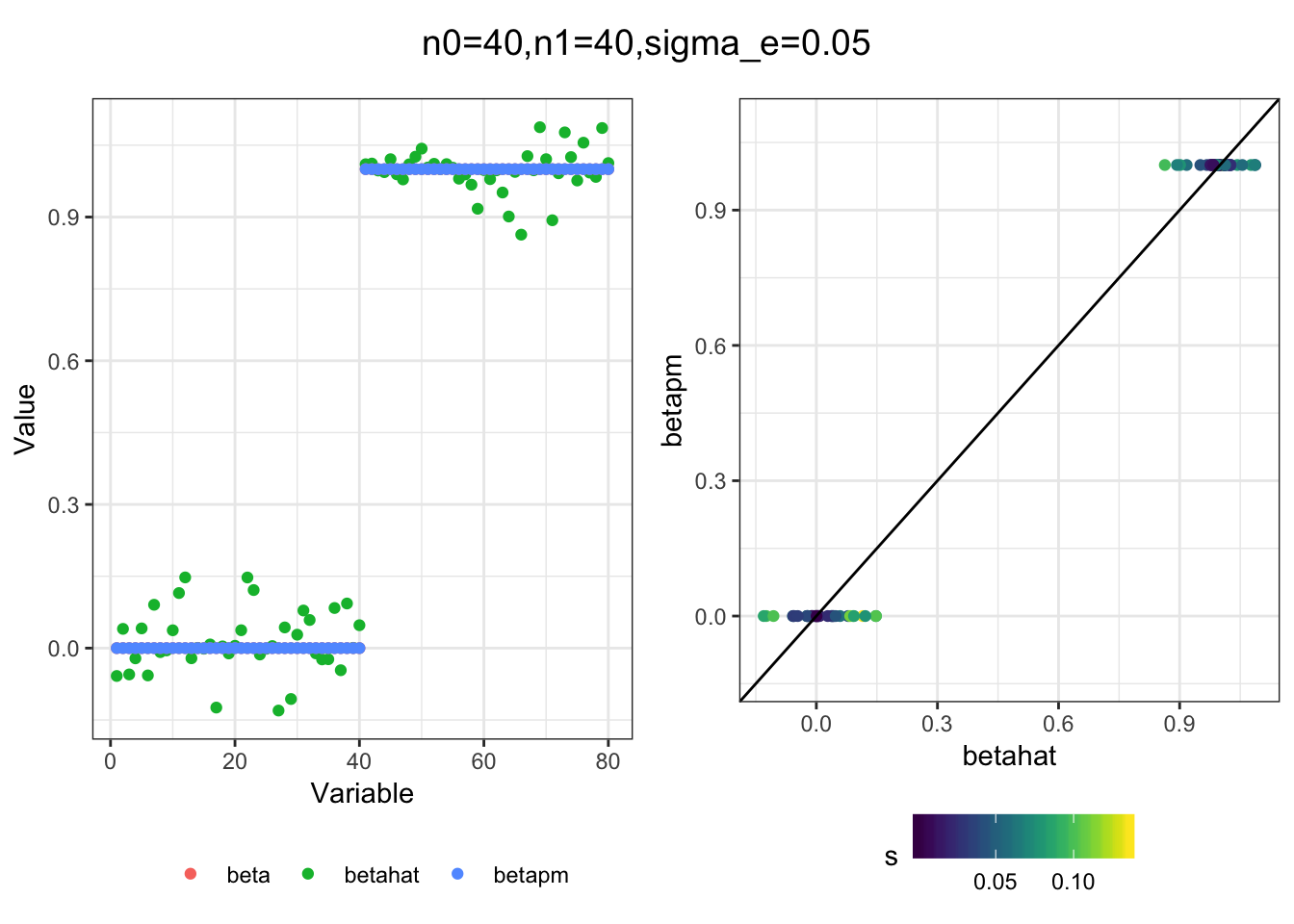
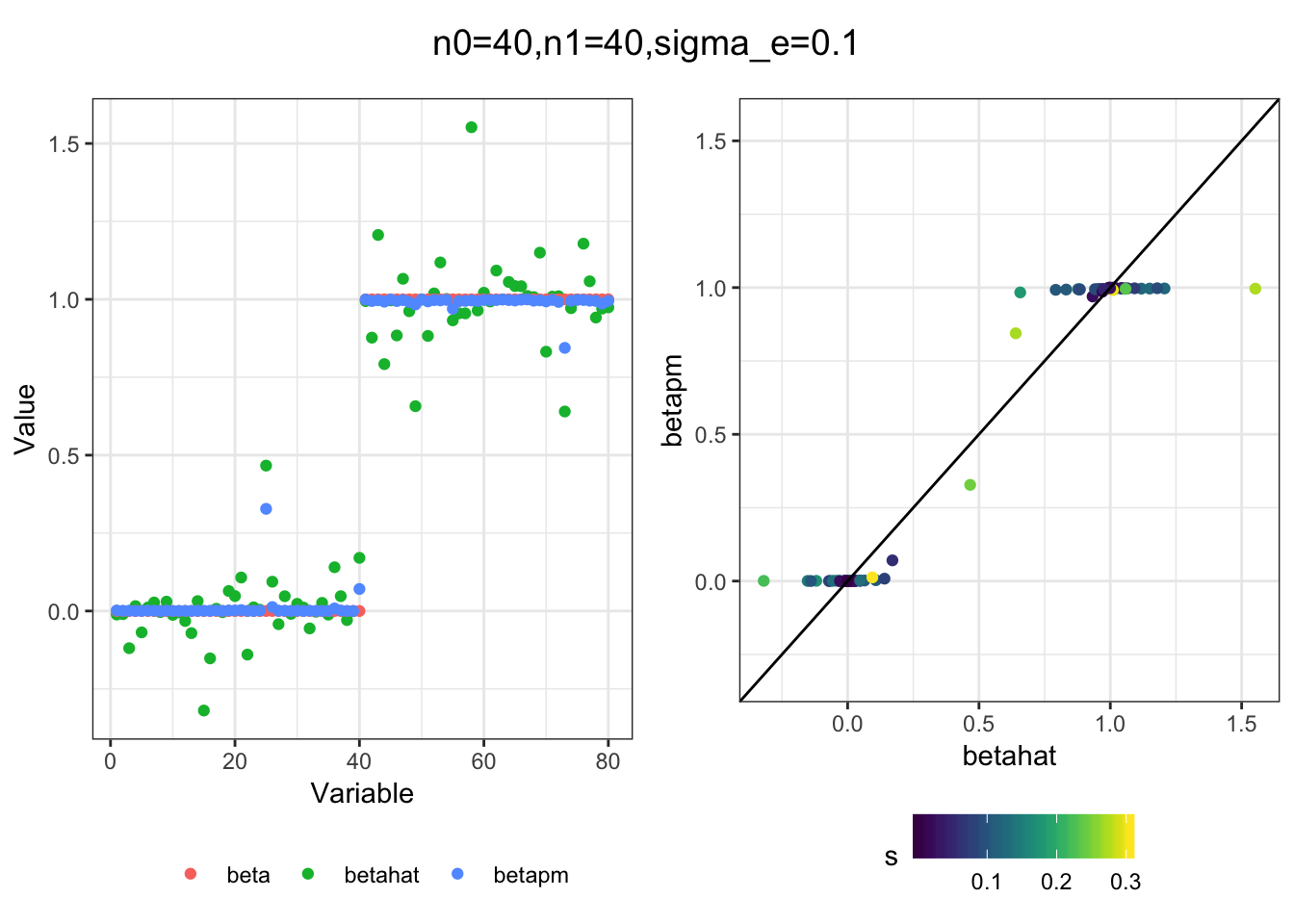
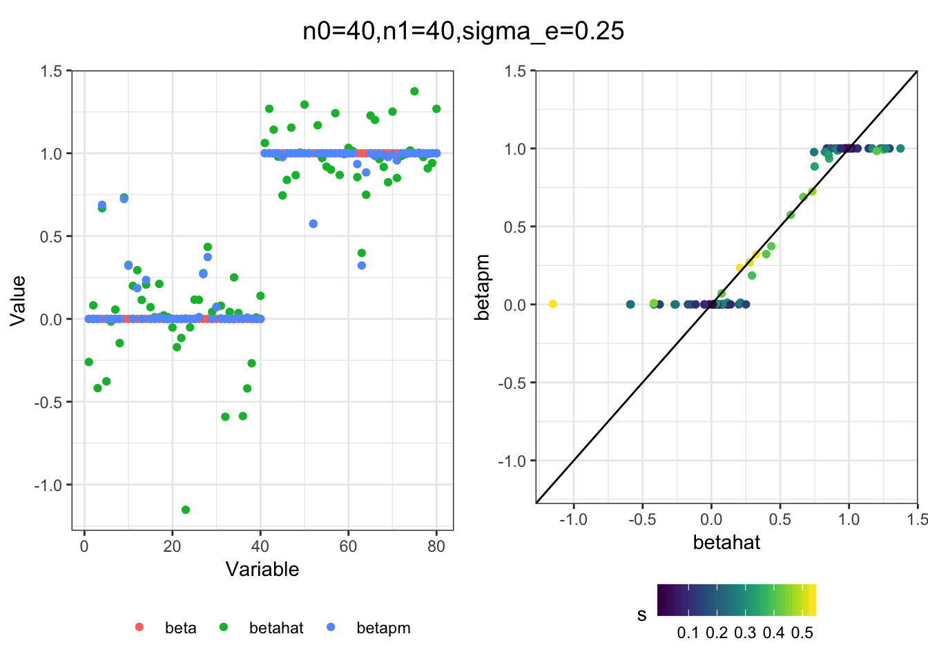
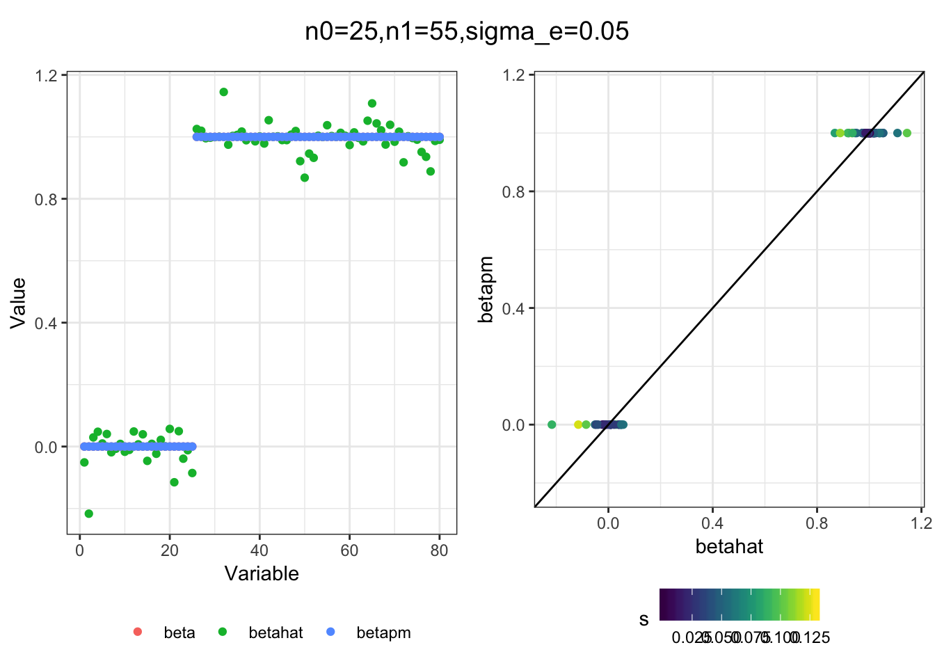
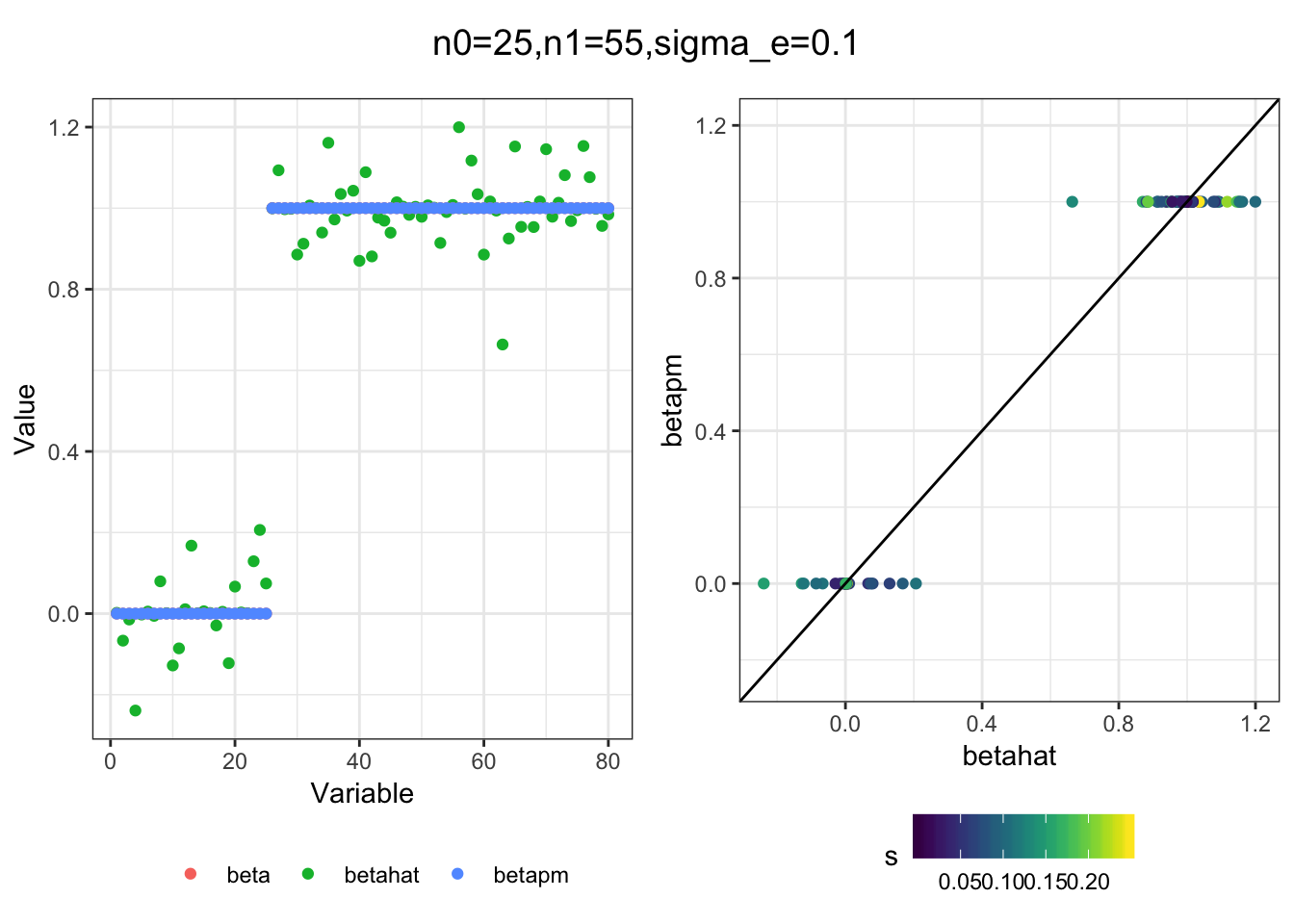
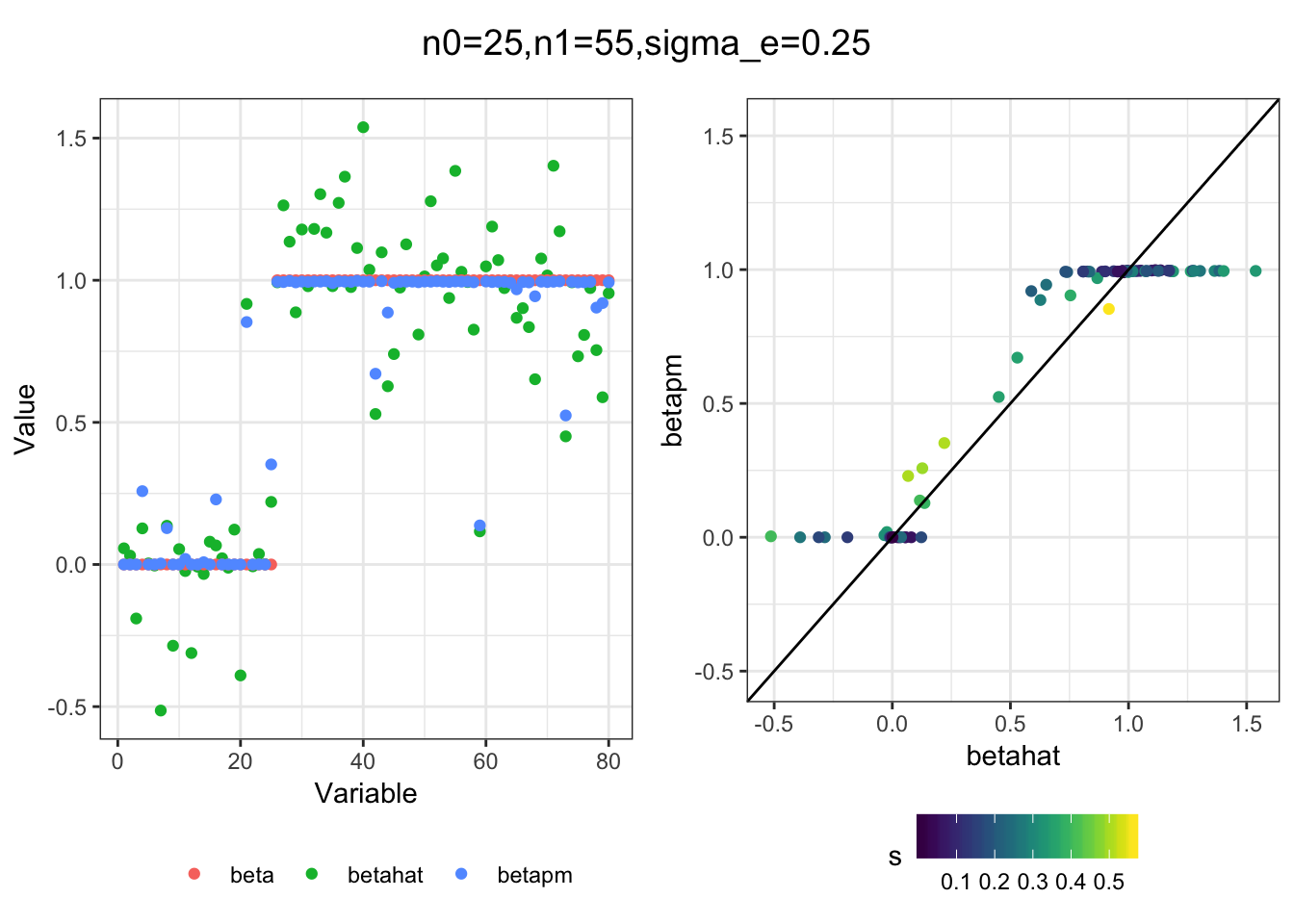
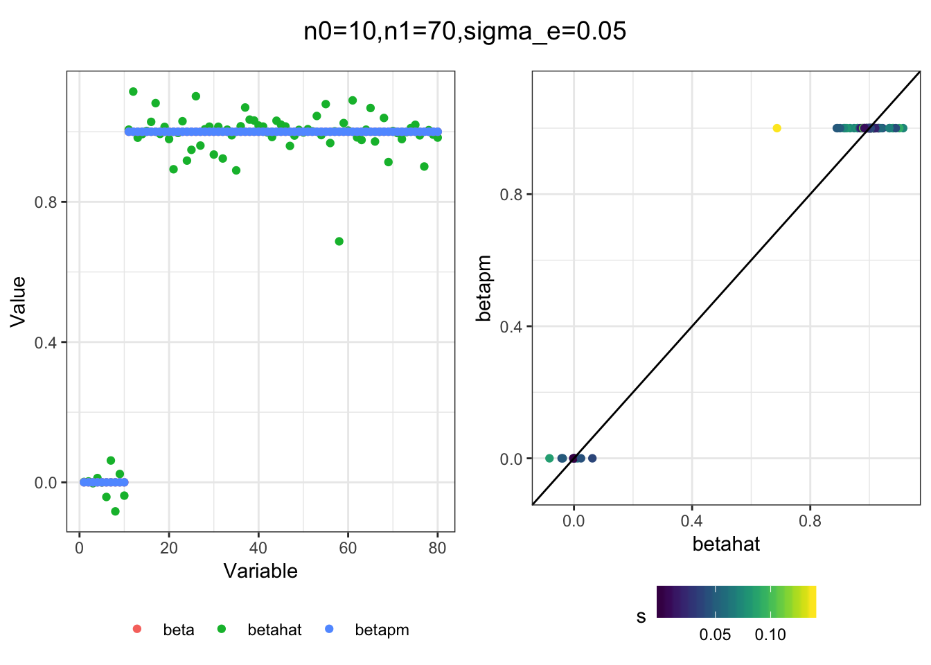

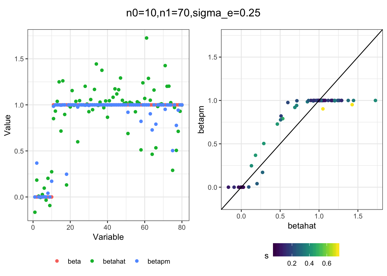
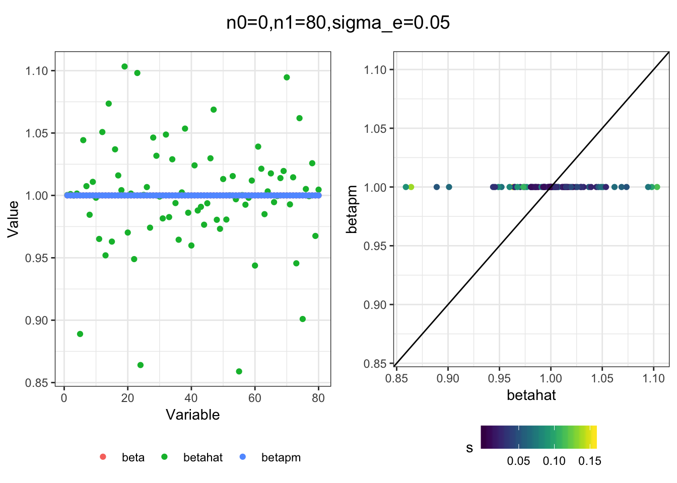
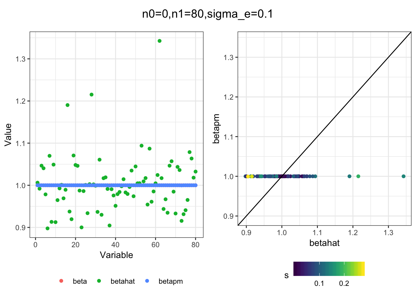
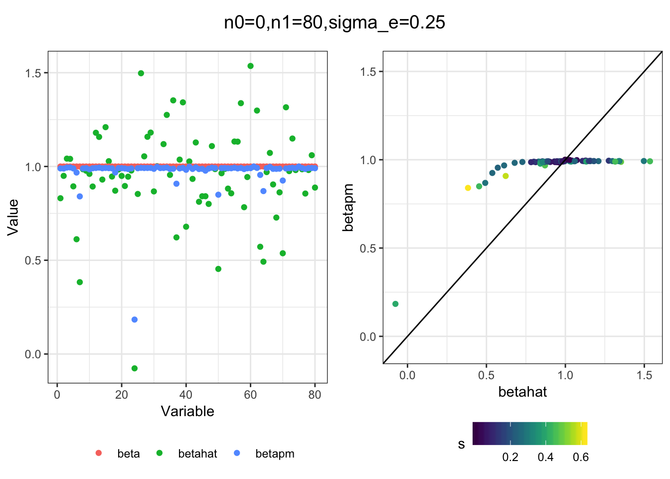
I think the idea roughly works! The most interesting scenarios to compare are when the std. errors of the estmates are high but the number of zeros and ones are different. Maybe we can define a term “bimodality” which I’m thinking is how bimodal the distribution is. When the bimodality is low (i.e. the prior distribution is closer to unimodal) the effects seem to be more correctly estimated. As we can see estimating more bimodal effects is a more difficult problem than unimodal effects.
It would also be interesting to think more about how to weight the prior mixture proportions if that would be helpful.
sessionInfo()R version 3.5.1 (2018-07-02)
Platform: x86_64-apple-darwin13.4.0 (64-bit)
Running under: macOS 10.14.2
Matrix products: default
BLAS/LAPACK: /Users/jhmarcus/miniconda3/lib/R/lib/libRblas.dylib
locale:
[1] en_US.UTF-8/en_US.UTF-8/en_US.UTF-8/C/en_US.UTF-8/en_US.UTF-8
attached base packages:
[1] stats graphics grDevices utils datasets methods base
other attached packages:
[1] tidyr_0.8.2 dplyr_0.8.0.1 ggplot2_3.1.0
loaded via a namespace (and not attached):
[1] Rcpp_1.0.0 compiler_3.5.1 pillar_1.3.1
[4] git2r_0.23.0 plyr_1.8.4 workflowr_1.2.0
[7] viridis_0.5.1 iterators_1.0.10 tools_3.5.1
[10] digest_0.6.18 viridisLite_0.3.0 lattice_0.20-38
[13] evaluate_0.12 tibble_2.0.1 gtable_0.2.0
[16] pkgconfig_2.0.2 rlang_0.3.1 foreach_1.4.4
[19] Matrix_1.2-15 parallel_3.5.1 yaml_2.2.0
[22] xfun_0.4 gridExtra_2.3 withr_2.1.2
[25] stringr_1.4.0 knitr_1.21 fs_1.2.6
[28] cowplot_0.9.4 rprojroot_1.3-2 grid_3.5.1
[31] tidyselect_0.2.5 glue_1.3.0 R6_2.4.0
[34] rmarkdown_1.11 mixsqp_0.1-115 purrr_0.3.0
[37] ashr_2.2-37 magrittr_1.5 whisker_0.3-2
[40] MASS_7.3-51.1 codetools_0.2-16 backports_1.1.3
[43] scales_1.0.0 htmltools_0.3.6 assertthat_0.2.0
[46] colorspace_1.4-0 labeling_0.3 stringi_1.2.4
[49] pscl_1.5.2 doParallel_1.0.14 lazyeval_0.2.1
[52] munsell_0.5.0 truncnorm_1.0-8 SQUAREM_2017.10-1
[55] crayon_1.3.4