Penalized drift: simple admixture event

Introduction

I attempted to use the methods described here to fit a four-population tree with an additional admixed Population E. I used admixture proportions of \(1/2\) for Population B, \(1/3\) for Population C, and \(1/6\) for Population D, so that individuals from Population E have data distributed \[ N \left( \frac{a + b + e}{2} + \frac{a + c + f}{3} + \frac{a + c + g}{6},\ \sigma^2_r I_p \right) \] I recovered the correct tree, but Population E was located at the root of the tree rather than showing up as an admixture. There are a number of fits that will achieve this result. For example:

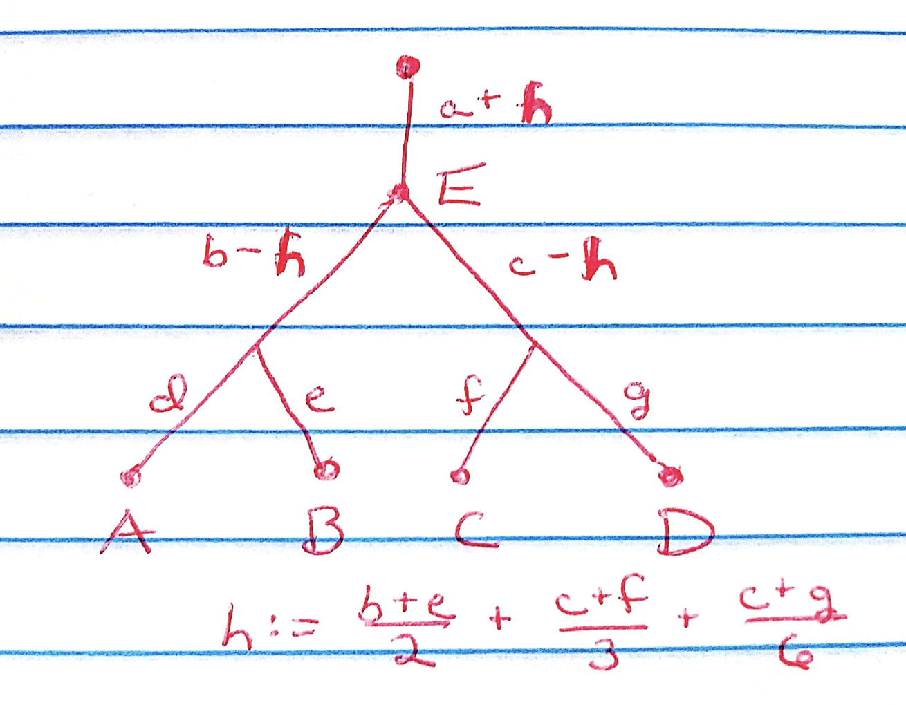
When I initialized to the true factors, I achieved a drift fit with a better ELBO, so this is once again an optimization issue rather than a problem with the objective function. But it’s very difficult to get from one optimum to the other, even if one knows in advance that Population E is an admixture and that the other populations are “pure.”

One way to detect the issue is to examine the cross-product \((EF)^T EF\). Since the “true” factors \(a, b, \ldots, g\) are mutually independent, the covariance matrix should be diagonal. It’s easy to see from the above diagram, however, that locating Population E at the root will result in nonzero off-diagonal entries.

In the analysis below I’ll consider the two-population admixture scenario, which distills the above difficulty. Indeed, if there are an equal number of individuals from Populations A and B and Population C is a 50-50 admixture, then the expected mean for Population C will be exactly equal to the expected sample mean. Since the greedy fit initializes the first factor at the sample mean, it will put Population C at the root of the tree, and it will be very difficult for drift to find its way out of that optimum.

Default fit

As expected, the default drift fit puts Population C at the root of the tree:

plot_dr <- function(dr) {
  sd <- sqrt(dr$prior_s2)
  L <- dr$EL
  LDsqrt <- L %*% diag(sd)
  K <- ncol(LDsqrt)
  plot_loadings(LDsqrt[,1:K], rep(c("A", "B", "C"), each = n_per_pop)) +
    scale_color_brewer(palette="Set2")
}

set.seed(666)

n_per_pop <- 60
p <- 10000

a <- rnorm(p)
b <- rnorm(p)
c <- rnorm(p)

popA <- c(rep(1, n_per_pop), rep(0, 2 * n_per_pop))
popB <- c(rep(0, n_per_pop), rep(1, n_per_pop), rep(0, n_per_pop))
popC <- c(rep(0, 2 * n_per_pop), rep(1, n_per_pop))

Y <- cbind(popA, popB, popC) %*% rbind(a + b, a + c, a + (b + c) / 2)
Y <- Y + rnorm(3 * n_per_pop * p, sd = 0.1)

dr_default <- drift(init_from_data(Y), verbose = FALSE)
plot_dr(dr_default)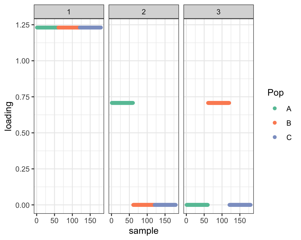

Since Factor 1 is approximately the sample mean \(a + \frac{b + c}{2}\), Factor 2 is approximately \(\frac{b - c}{2}\), while Factor 3 is approximately \(\frac{c - b}{2}\). Thus we observe a strong negative correlation between Factors 2 and 3:

plot_cov(cov(dr_default$EF), as.is = TRUE)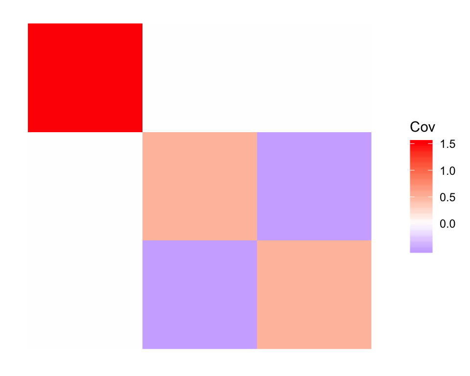

True factors

Next I initialize using the true factors. This initialization yields a better ELBO and clearly shows that Population C is an admixture:

true_EF <- cbind(a, b, c)
true_EL <- cbind(popA + popB + popC, popA + popC / 2, popB + popC / 2)

dr_true <- drift(init_from_EL(Y, EL = true_EL, EF = true_EF), miniter = 2, verbose = FALSE)

cat("ELBO (default initialization):", dr_default$elbo,
    "\nELBO (initialize from truth): ", dr_true$elbo)

#> ELBO (default initialization): 1465294 
#> ELBO (initialize from truth):  1495564

plot_dr(dr_true)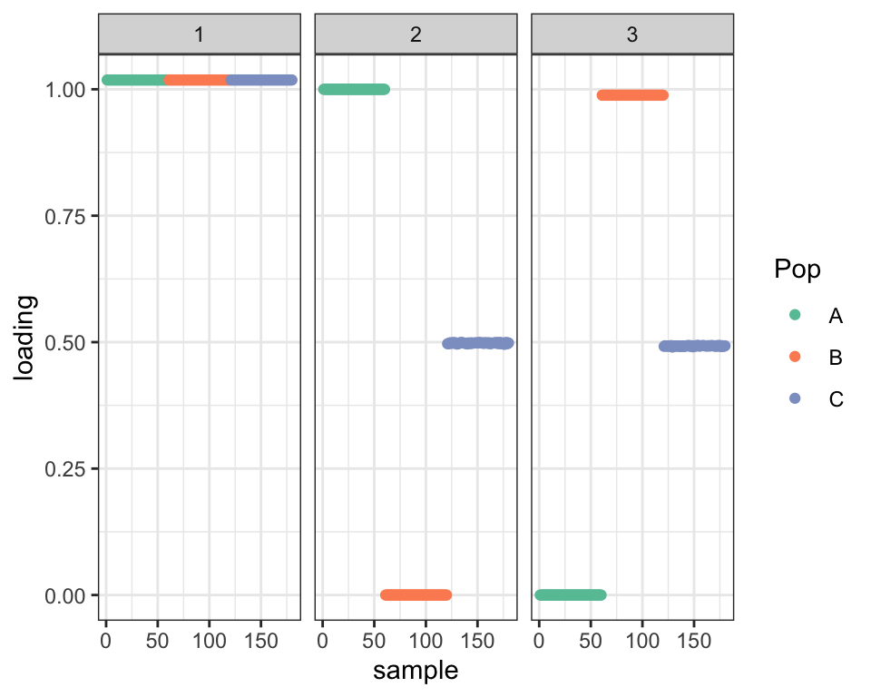

Note that this fit departs significantly from the initialization in that the off-diagonal entries of the covariance matrix are not particularly close to zero:

plot_cov(cov(dr_true$EF), as.is = TRUE)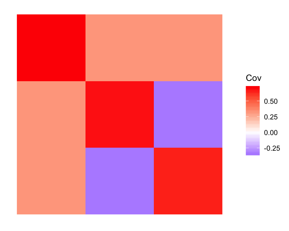

Penalized drift

To encourage drift to find optima where factors are orthogonal, I added a penalty to the objective function: \[ -\lambda \sum_{k, \ell: k \ne \ell} \left((EF_k)^T(EF_\ell) \right)^2\]

If I initialize using the true factors, Population C still shows up as an admixture, but now the factors are orthogonal:

dr_ortho <- drift(init_from_EL(Y, EL = true_EL, EF = true_EF), lambda = 10, 
                  miniter = 5, maxiter = 1000, verbose = FALSE)
plot_dr(dr_ortho)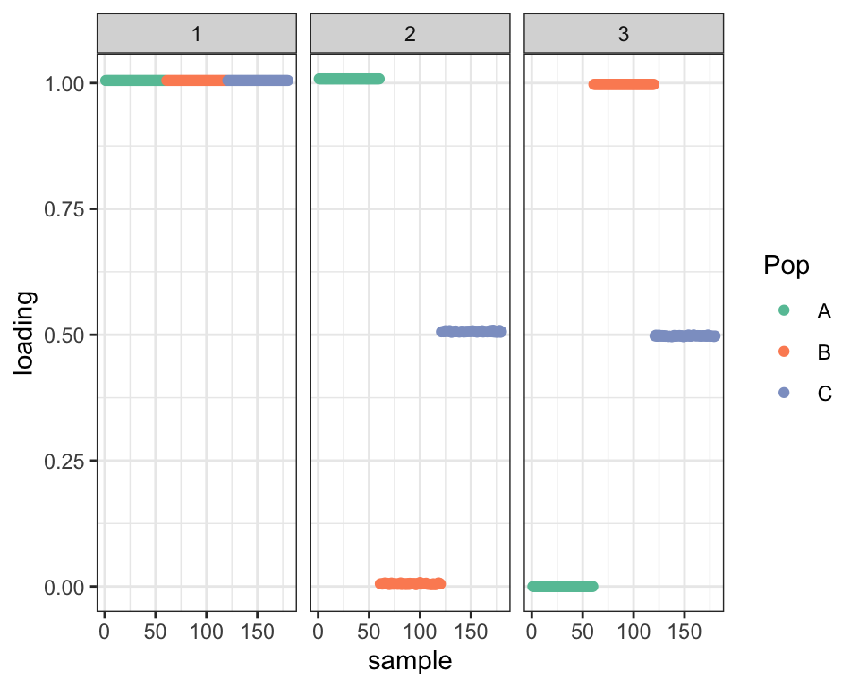

plot_cov(cov(dr_ortho$EF), as.is = TRUE)

Indeed, the fitted factors maintain the true factors almost exactly:

cor(dr_ortho$EF, cbind(true_a = a, true_b = b, true_c = c))

#>        true_a       true_b       true_c
#> a 0.999895497  0.005255480  0.005430503
#> b 0.008181082  0.999909023 -0.003200754
#> c 0.003296122 -0.003463083  0.999894953

This last result is perhaps not surprising, since that’s where the factors started. More surprisingly, I can recover the true factors if I start from the drift fit that was initialized from the truth (which, recall, departed significantly from the initialization):

dr_ortho2 <- drift(init_from_EL(Y, EL = dr_ortho$EL, EF = dr_ortho$EF), lambda = 10, 
                  miniter = 5, maxiter = 1000, verbose = FALSE)
cor(dr_ortho2$EF, cbind(true_a = a, true_b = b, true_c = c))

#>        true_a       true_b       true_c
#> a 0.999828791  0.006028031  0.006231853
#> b 0.007552972  0.999833392 -0.003978480
#> c 0.002648496 -0.002843890  0.999814502

Penalized drift with greedy initialization

Another encouraging result is that drift is able to find the admixture when I use the default initialization (which, as I argued above, should be a very difficult optimum to escape). In fact, the default initialization finds an even better solution (judging by the penalized ELBO):

# I need to gently ramp up lambda in order for this to work:
dr_greedy_ortho <- drift(init_from_data(Y), 
                         lambda = 1, miniter = 5, maxiter = 1000, verbose = FALSE)
dr_greedy_ortho <- drift(init_from_EL(Y, EL = dr_greedy_ortho$EL, EF = dr_greedy_ortho$EF),
                         lambda = 10, miniter = 5, maxiter = 1000, verbose = FALSE)

cat("Penalized ELBO (default initialization):", dr_greedy_ortho$elbo,
    "\nPenalized ELBO (initialize from truth): ", dr_ortho$elbo)

#> Penalized ELBO (default initialization): 1451299 
#> Penalized ELBO (initialize from truth):  1446707

plot_dr(dr_greedy_ortho)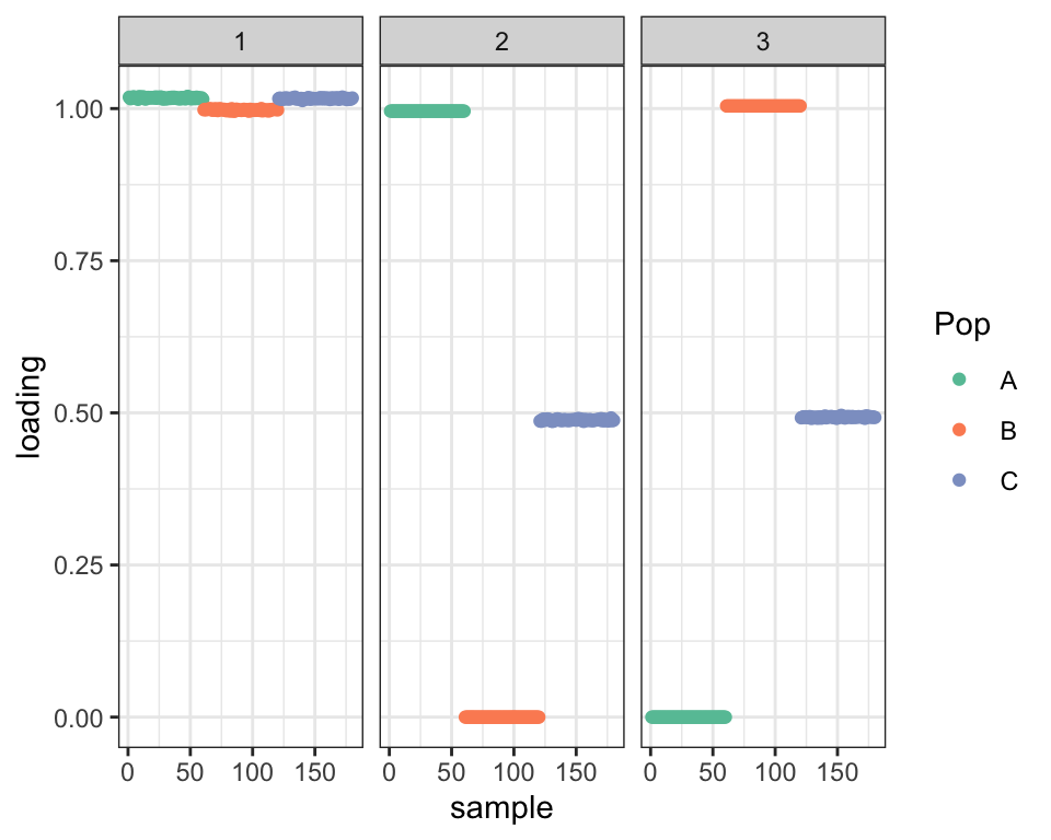

plot_cov(cov(dr_greedy_ortho$EF), as.is = TRUE)

Since, in theory, the drift objective encourages orthogonality, my intention was to use the penalized approach to find a good initialization and then to re-run drift without the penalty. Doing so retains the admixture but re-introduces some covariance (which is similar to the covariance in the fit that was initialized using the true factors):

dr_pen_init <- drift(init_from_EL(Y, EL = dr_greedy_ortho$EL, EF = dr_greedy_ortho$EF),
                      lambda = 0, miniter = 5, maxiter = 1000, verbose = FALSE)
plot_dr(dr_pen_init)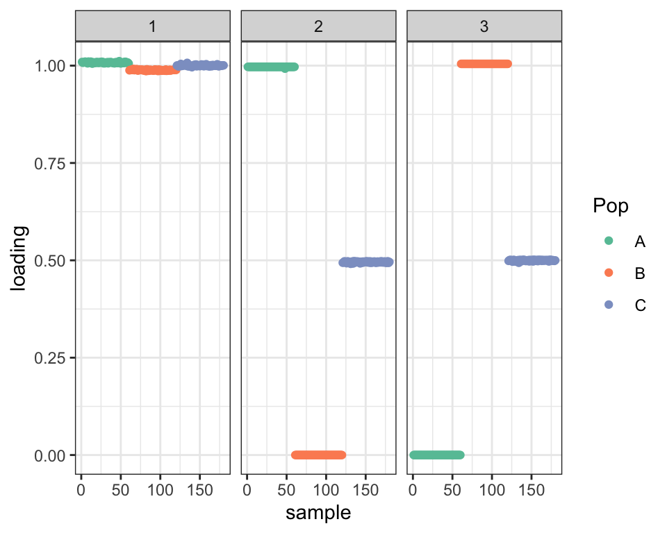

plot_cov(cov(dr_pen_init$EF), as.is = TRUE)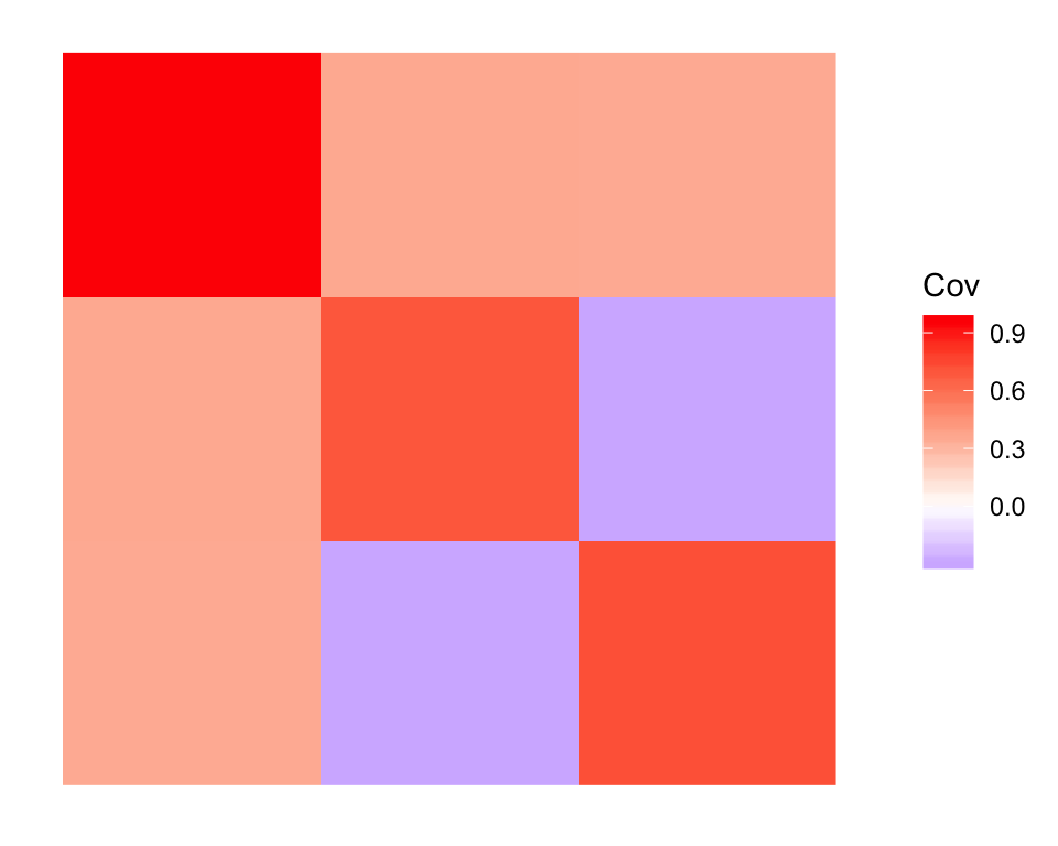

The ELBO is not as good as when I initialize using the true factors, but it’s not nearly as far off as it was when I used the default greedy initialization:

cat("ELBO (orthogonal initialization):", dr_pen_init$elbo,
    "\nELBO (initialize from truth):    ", dr_true$elbo)

#> ELBO (orthogonal initialization): 1494914 
#> ELBO (initialize from truth):     1495564

Conclusion

Using a penalized approach that encourages orthogonal factors, I was able to find the admixture even in this very difficult scenario where the mean of the admixed population is equal to the overall population mean. Further, the penalized approach can recover the true factors nearly exactly if the initialization is close enough to the truth.

Session information

sessionInfo()

#> R version 3.5.3 (2019-03-11)
#> Platform: x86_64-apple-darwin15.6.0 (64-bit)
#> Running under: macOS Mojave 10.14.6
#> 
#> Matrix products: default
#> BLAS: /Library/Frameworks/R.framework/Versions/3.5/Resources/lib/libRblas.0.dylib
#> LAPACK: /Library/Frameworks/R.framework/Versions/3.5/Resources/lib/libRlapack.dylib
#> 
#> locale:
#> [1] en_US.UTF-8/en_US.UTF-8/en_US.UTF-8/C/en_US.UTF-8/en_US.UTF-8
#> 
#> attached base packages:
#> [1] stats     graphics  grDevices utils     datasets  methods   base     
#> 
#> other attached packages:
#>  [1] forcats_0.4.0     stringr_1.4.0     dplyr_0.8.0.1    
#>  [4] purrr_0.3.2       readr_1.3.1       tidyr_0.8.3      
#>  [7] tibble_2.1.1      ggplot2_3.2.0     tidyverse_1.2.1  
#> [10] drift.alpha_0.0.9 flashier_0.2.4   
#> 
#> loaded via a namespace (and not attached):
#>  [1] Rcpp_1.0.4.6       lubridate_1.7.4    invgamma_1.1      
#>  [4] lattice_0.20-38    assertthat_0.2.1   rprojroot_1.3-2   
#>  [7] digest_0.6.18      truncnorm_1.0-8    R6_2.4.0          
#> [10] cellranger_1.1.0   plyr_1.8.4         backports_1.1.3   
#> [13] evaluate_0.13      httr_1.4.0         pillar_1.3.1      
#> [16] rlang_0.4.2        lazyeval_0.2.2     readxl_1.3.1      
#> [19] rstudioapi_0.10    ebnm_0.1-21        irlba_2.3.3       
#> [22] whisker_0.3-2      Matrix_1.2-15      rmarkdown_1.12    
#> [25] labeling_0.3       munsell_0.5.0      mixsqp_0.3-40     
#> [28] broom_0.5.1        compiler_3.5.3     modelr_0.1.5      
#> [31] xfun_0.6           pkgconfig_2.0.2    SQUAREM_2017.10-1 
#> [34] htmltools_0.3.6    tidyselect_0.2.5   workflowr_1.2.0   
#> [37] withr_2.1.2        crayon_1.3.4       grid_3.5.3        
#> [40] nlme_3.1-137       jsonlite_1.6       gtable_0.3.0      
#> [43] git2r_0.25.2       magrittr_1.5       scales_1.0.0      
#> [46] cli_1.1.0          stringi_1.4.3      reshape2_1.4.3    
#> [49] fs_1.2.7           xml2_1.2.0         generics_0.0.2    
#> [52] RColorBrewer_1.1-2 tools_3.5.3        glue_1.3.1        
#> [55] hms_0.4.2          parallel_3.5.3     yaml_2.2.0        
#> [58] colorspace_1.4-1   ashr_2.2-50        rvest_0.3.4       
#> [61] knitr_1.22         haven_2.1.1