Revisiting prior families for trees
Jason Willwerscheid
7/22/2020
Last updated: 2020-07-22
Checks: 6 0
Knit directory: drift-workflow/analysis/
This reproducible R Markdown analysis was created with workflowr (version 1.2.0). The Report tab describes the reproducibility checks that were applied when the results were created. The Past versions tab lists the development history.
Great! Since the R Markdown file has been committed to the Git repository, you know the exact version of the code that produced these results.
Great job! The global environment was empty. Objects defined in the global environment can affect the analysis in your R Markdown file in unknown ways. For reproduciblity it’s best to always run the code in an empty environment.
The command set.seed(20190211) was run prior to running the code in the R Markdown file. Setting a seed ensures that any results that rely on randomness, e.g. subsampling or permutations, are reproducible.
Great job! Recording the operating system, R version, and package versions is critical for reproducibility.
Nice! There were no cached chunks for this analysis, so you can be confident that you successfully produced the results during this run.
Great! You are using Git for version control. Tracking code development and connecting the code version to the results is critical for reproducibility. The version displayed above was the version of the Git repository at the time these results were generated.
Note that you need to be careful to ensure that all relevant files for the analysis have been committed to Git prior to generating the results (you can use wflow_publish or wflow_git_commit). workflowr only checks the R Markdown file, but you know if there are other scripts or data files that it depends on. Below is the status of the Git repository when the results were generated:
Ignored files:
    Ignored:    .DS_Store
    Ignored:    .Rhistory
    Ignored:    .Rproj.user/
    Ignored:    docs/.DS_Store
    Ignored:    docs/assets/.DS_Store
    Ignored:    output/

Untracked files:
    Untracked:  analysis/extrapolate3.Rmd
    Untracked:  analysis/extrapolate4.Rmd

Unstaged changes:
    Modified:   drift-workflow.Rproj
Note that any generated files, e.g. HTML, png, CSS, etc., are not included in this status report because it is ok for generated content to have uncommitted changes.
These are the previous versions of the R Markdown and HTML files. If you’ve configured a remote Git repository (see ?wflow_git_remote), click on the hyperlinks in the table below to view them.
| File | Version | Author | Date | Message |
|---|---|---|---|---|
| Rmd | bdd4361 | Jason Willwerscheid | 2020-07-22 | workflowr::wflow_publish(“analysis/pm1_priors.Rmd”) |
suppressMessages({
  library(flashier)
  library(drift.alpha)
  library(tidyverse)
})
I use the four-population tree that I also used in my exploration of random initialization.
set.seed(666)

n_per_pop <- 60
p <- 10000

a <- rnorm(p)
b <- rnorm(p)
c <- rnorm(p)
d <- rnorm(p, sd = 0.5)
e <- rnorm(p, sd = 0.5)
f <- rnorm(p, sd = 0.5)
g <- rnorm(p, sd = 0.5)

popA <- c(rep(1, n_per_pop), rep(0, 4 * n_per_pop))
popB <- c(rep(0, n_per_pop), rep(1, n_per_pop), rep(0, 3 * n_per_pop))
popC <- c(rep(0, 2 * n_per_pop), rep(1, n_per_pop), rep(0, 2 * n_per_pop))
popD <- c(rep(0, 3 * n_per_pop), rep(1, n_per_pop), rep(0, n_per_pop))
popE <- c(rep(0, 4 * n_per_pop), rep(1, n_per_pop))

E.factor <- (a + b + e) / 2 + (a + c + f) / 3 + (a + c + g) / 6

Y <- cbind(popA, popB, popC, popD, popE) %*%
  rbind(a + b + d, a + b + e, a + c + f, a + c + g, E.factor)
Y <- Y + rnorm(5 * n_per_pop * p, sd = 0.1)

plot_dr <- function(dr) {
  sd <- sqrt(dr$prior_s2)
  L <- dr$EL
  LDsqrt <- L %*% diag(sd)
  K <- ncol(LDsqrt)
  plot_loadings(LDsqrt[,1:K], rep(c("A", "B", "C", "D", "E"), each = n_per_pop)) +
    scale_color_brewer(palette="Set2")
}
We should be able to get to a factorization where each column corresponds to a split in a tree: \[ \begin{bmatrix} 1 & 1 & 1 & 0 \\ 1 & 1 & -1 & 0 \\ 1 & -1 & 0 & 1 \\ 1 & -1 & 0 & -1 \\ 1 & 0 & -1/2 & 1/6 \end{bmatrix} \begin{bmatrix} f_1 \\ f_2 \\ f_3 \\ f_4 \end{bmatrix} \] The first column in the matrix on the left corresponds to the root; the second, to the top split; and the third and fourth, to the bottom splits. Since this matrix is full rank, we might expect that this solution would be easier to find than the solutions we want to get from the bimodal priors we’ve been using so far. (The last row corresponds to the admixed population \(E\): for example, since it is half population \(B\) and half populations \(C\) and \(D\), it shares equally in both sides of the top split, so its entry in the second column is \(1/2 - 1/2 = 0\).)
To try to obtain such a factorization, I try to use mixtures of a pointmass at -1, a pointmass at +1, and a uniform component in between.
tree.fn = function(x, s, g_init, fix_g, output, ...) {
  if (is.null(g_init)) {
    g_init <- ashr::unimix(rep(1/3, 3), c(-1, -1, 1), c(-1, 1, 1))
  }

  return(flashier:::ebnm.nowarn(x = x,
                                s = s,
                                g_init = g_init,
                                fix_g = fix_g,
                                output = output,
                                prior_family = "ash",
                                prior = c(10, 1, 10),
                                ...))
}

prior.tree = function(...) {
  return(as.prior(sign = 0, ebnm.fn = function(x, s, g_init, fix_g, output) {
    tree.fn(x, s, g_init, fix_g, output, ...)
  }))
}
First I fit a vector of ones (the root) and then I fit the top split by adding a “greedy” factor:
ones <- matrix(1, nrow = nrow(Y), ncol = 1)
ls.soln <- t(solve(crossprod(ones), crossprod(ones, Y)))

fl <- flash.init(Y) %>%
  flash.set.verbose(0) %>%
  flash.init.factors(EF = list(ones, ls.soln),
                     prior.family = c(prior.tree(), prior.normal())) %>%
  flash.fix.loadings(kset = 1, mode = 1L) %>%
  flash.backfit() %>%
  flash.add.greedy(prior.family = c(prior.tree(), prior.normal())) %>%
  flash.backfit()
plot(fl$flash.fit$EF[[1]][, 2])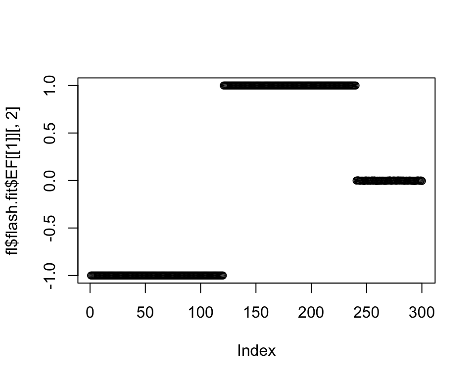
So far, so good. To fit the next two branches, we have two options: either remove the individuals that don’t fit nicely (Population E) from the next two splits (and re-fit later) or allow them to be loaded on both splits. In either case, the loadings of the individuals from the opposite side of the split should be fixed at zero. I try the first method first (one side of the split only):
set1 <- (fl$flash.fit$EF[[1]][, 2] > 0.9)
set2 <- (fl$flash.fit$EF[[1]][, 2] < -0.9)
set3 <- !set1 & !set2 # admixed individuals

next.factor <- matrix(1L * set1, ncol = 1)
ls.soln <- t(solve(crossprod(next.factor), crossprod(next.factor, Y)))

fl2 <- fl %>%
  flash.init.factors(EF = list(next.factor, ls.soln),
                     prior.family = c(prior.tree(), prior.normal())) %>%
  flash.fix.loadings(kset = 3, mode = 1L) %>%
  flash.backfit(3)

next.factor <- matrix(sample(c(-1, 1), size = nrow(Y), replace = TRUE) * set1, ncol = 1)
ls.soln <- t(solve(crossprod(next.factor), crossprod(next.factor, Y)))

fl2 <- fl2 %>%
  flash.init.factors(EF = list(next.factor, ls.soln),
                     prior.family = c(prior.tree(), prior.normal())) %>%
  flash.fix.loadings(kset = 4, mode = 1L, is.fixed = set2 | set3) %>%
  flash.backfit(4)

plot(fl2$flash.fit$EF[[1]][, 4])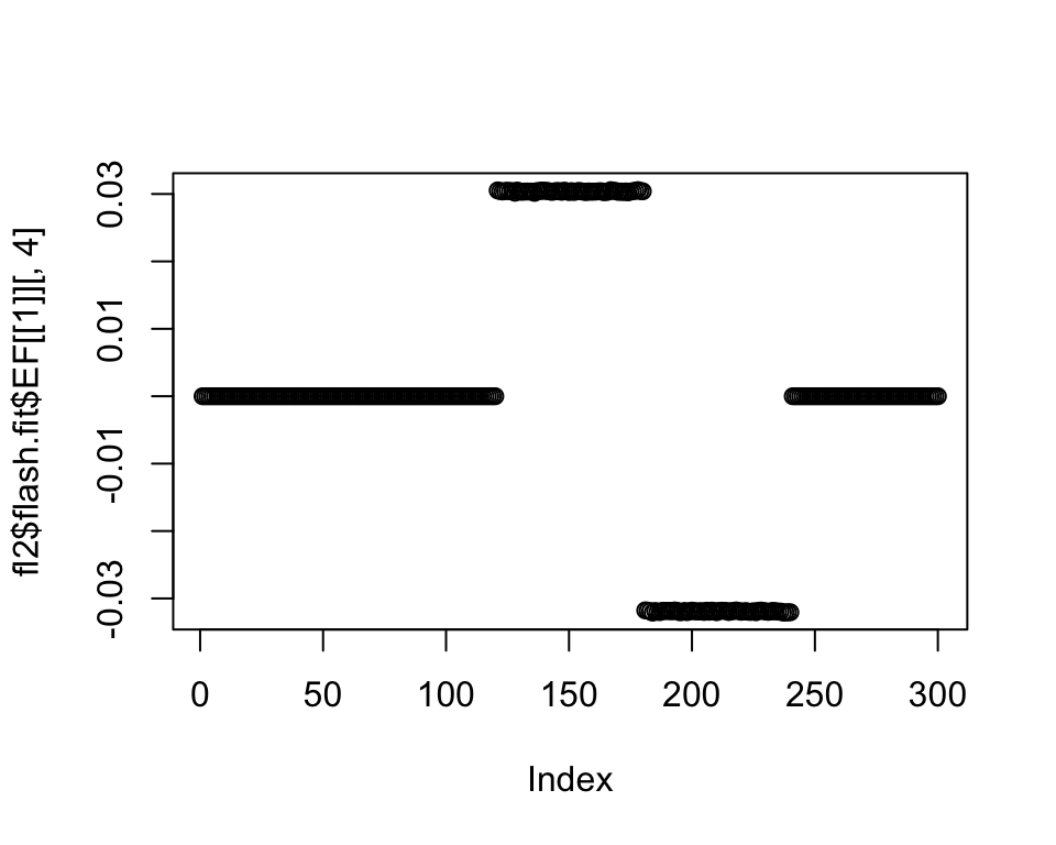
I don’t know why a solution loaded on -1 and +1 isn’t preferred (or, even if the loadings aren’t exactly symmetric, I’d at least expect it to be loaded on one of the two poles). We might need to think about the prior family some more. For example, an NPMLE prior can capture the fact that the loadings should be distributed as a small number of pointmasses:
npmle.fn = function(x, s, g_init, fix_g, output, ...) {
  return(flashier:::ebnm.nowarn(x = x,
                                s = s,
                                g_init = g_init,
                                fix_g = fix_g,
                                output = output,
                                prior_family = "npmle",
                                ...))
}

prior.npmle = function(...) {
  return(as.prior(sign = 0, ebnm.fn = function(x, s, g_init, fix_g, output) {
    npmle.fn(x, s, g_init, fix_g, output, ...)
  }))
}

ones <- matrix(1, nrow = nrow(Y), ncol = 1)
ls.soln <- t(solve(crossprod(ones), crossprod(ones, Y)))

fl <- flash.init(Y) %>%
  flash.set.verbose(0) %>%
  flash.init.factors(EF = list(ones, ls.soln),
                     prior.family = c(prior.npmle(), prior.normal())) %>%
  flash.fix.loadings(kset = 1, mode = 1L) %>%
  flash.backfit() %>%
  flash.add.greedy(prior.family = c(prior.npmle(), prior.normal())) %>%
  flash.backfit(warmstart = FALSE)
plot(fl$flash.fit$EF[[1]][, 2])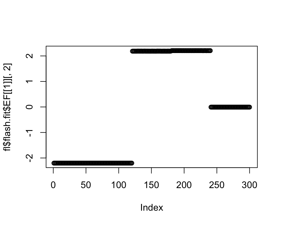
set1 <- popA | popB
set2 <- popC | popD
set3 <- popE

next.factor <- matrix(1L * set1, ncol = 1)
ls.soln <- t(solve(crossprod(next.factor), crossprod(next.factor, Y)))

fl2 <- fl %>%
  flash.init.factors(EF = list(next.factor, ls.soln),
                     prior.family = c(prior.npmle(), prior.normal())) %>%
  flash.fix.loadings(kset = 3, mode = 1L) %>%
  flash.backfit(3)

next.factor <- matrix(sample(c(-1, 1), size = nrow(Y), replace = TRUE) * set1, ncol = 1)
ls.soln <- t(solve(crossprod(next.factor), crossprod(next.factor, Y)))

fl2 <- fl2 %>%
  flash.init.factors(EF = list(next.factor, ls.soln),
                     prior.family = c(prior.npmle(), prior.normal())) %>%
  flash.fix.loadings(kset = 4, mode = 1L, is.fixed = set2 | set3) %>%
  flash.backfit(4, warmstart = FALSE)

plot(fl2$flash.fit$EF[[1]][, 4])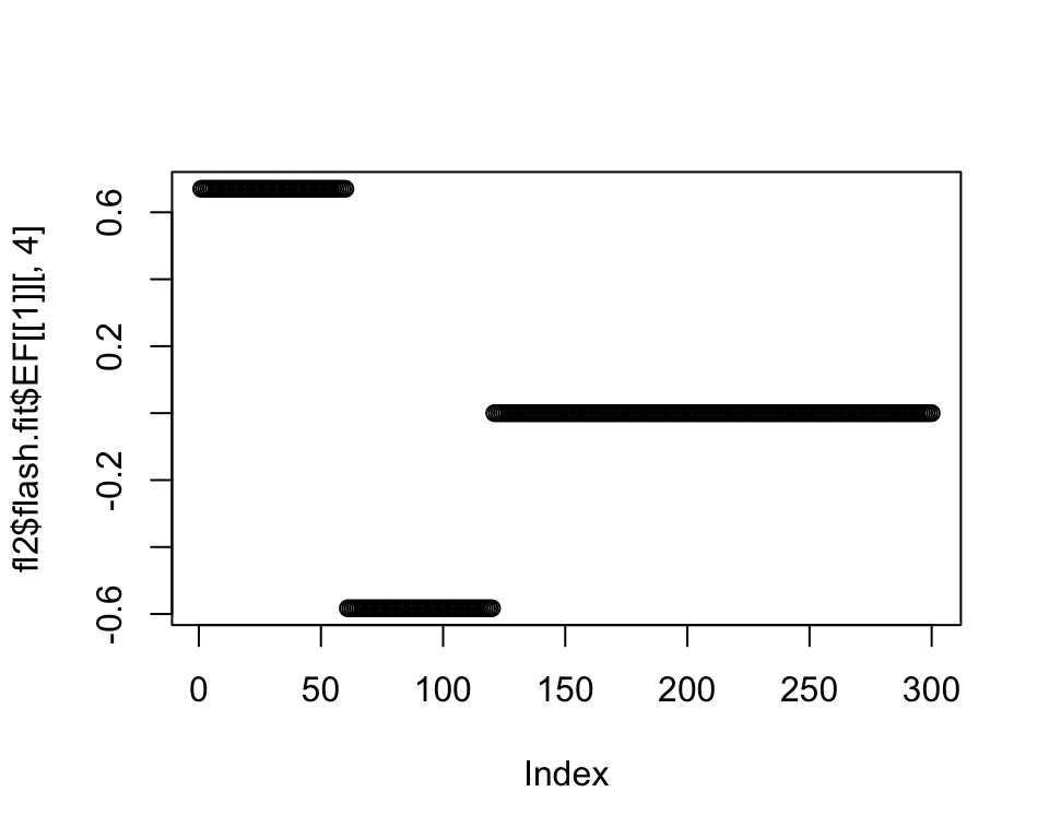
If I allow Population E to be included in this factor, I get:
next.factor <- matrix(1L * set1, ncol = 1)
ls.soln <- t(solve(crossprod(next.factor), crossprod(next.factor, Y)))

fl2 <- fl %>%
  flash.init.factors(EF = list(next.factor, ls.soln),
                     prior.family = c(prior.npmle(), prior.normal())) %>%
  flash.fix.loadings(kset = 3, mode = 1L) %>%
  flash.backfit(3)

next.factor <- matrix(sample(c(-1, 1), size = nrow(Y), replace = TRUE) * (set1 | set3), ncol = 1)
ls.soln <- t(solve(crossprod(next.factor), crossprod(next.factor, Y)))

fl2 <- fl2 %>%
  flash.init.factors(EF = list(next.factor, ls.soln),
                     prior.family = c(prior.npmle(), prior.normal())) %>%
  flash.fix.loadings(kset = 4, mode = 1L, is.fixed = set2) %>%
  flash.backfit(4, warmstart = FALSE)

plot(fl2$flash.fit$EF[[1]][, 4])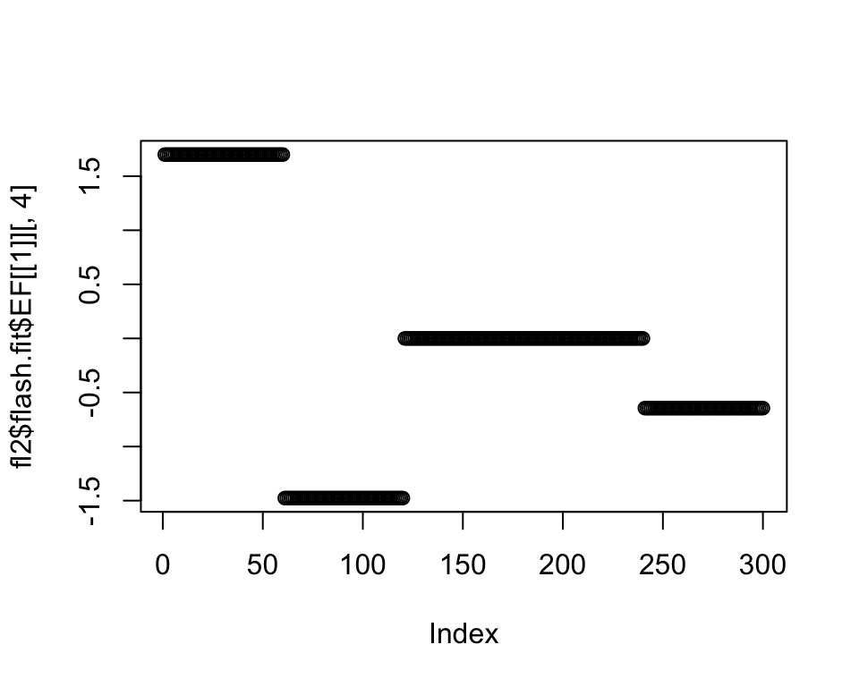
sessionInfo()#> R version 3.5.3 (2019-03-11)
#> Platform: x86_64-apple-darwin15.6.0 (64-bit)
#> Running under: macOS Mojave 10.14.6
#>
#> Matrix products: default
#> BLAS: /Library/Frameworks/R.framework/Versions/3.5/Resources/lib/libRblas.0.dylib
#> LAPACK: /Library/Frameworks/R.framework/Versions/3.5/Resources/lib/libRlapack.dylib
#>
#> locale:
#> [1] en_US.UTF-8/en_US.UTF-8/en_US.UTF-8/C/en_US.UTF-8/en_US.UTF-8
#>
#> attached base packages:
#> [1] stats graphics grDevices utils datasets methods base
#>
#> other attached packages:
#> [1] forcats_0.4.0 stringr_1.4.0 dplyr_0.8.0.1
#> [4] purrr_0.3.2 readr_1.3.1 tidyr_0.8.3
#> [7] tibble_2.1.1 ggplot2_3.2.0 tidyverse_1.2.1
#> [10] drift.alpha_0.0.9 flashier_0.2.4
#>
#> loaded via a namespace (and not attached):
#> [1] Rcpp_1.0.4.6 lubridate_1.7.4 invgamma_1.1
#> [4] lattice_0.20-38 assertthat_0.2.1 rprojroot_1.3-2
#> [7] digest_0.6.18 truncnorm_1.0-8 R6_2.4.0
#> [10] cellranger_1.1.0 plyr_1.8.4 backports_1.1.3
#> [13] evaluate_0.13 httr_1.4.0 pillar_1.3.1
#> [16] rlang_0.4.2 lazyeval_0.2.2 readxl_1.3.1
#> [19] rstudioapi_0.10 ebnm_0.1-21 irlba_2.3.3
#> [22] whisker_0.3-2 Matrix_1.2-15 rmarkdown_1.12
#> [25] munsell_0.5.0 mixsqp_0.3-40 broom_0.5.1
#> [28] compiler_3.5.3 modelr_0.1.5 xfun_0.6
#> [31] pkgconfig_2.0.2 SQUAREM_2017.10-1 htmltools_0.3.6
#> [34] tidyselect_0.2.5 workflowr_1.2.0 withr_2.1.2
#> [37] crayon_1.3.4 grid_3.5.3 nlme_3.1-137
#> [40] jsonlite_1.6 gtable_0.3.0 git2r_0.25.2
#> [43] magrittr_1.5 scales_1.0.0 cli_1.1.0
#> [46] stringi_1.4.3 reshape2_1.4.3 fs_1.2.7
#> [49] xml2_1.2.0 generics_0.0.2 tools_3.5.3
#> [52] glue_1.3.1 hms_0.4.2 parallel_3.5.3
#> [55] yaml_2.2.0 colorspace_1.4-1 ashr_2.2-51
#> [58] rvest_0.3.4 knitr_1.22 haven_2.1.1