Revisiting prior families for trees: Part II

workflowr

Ignored files:
    Ignored:    .DS_Store
    Ignored:    .Rhistory
    Ignored:    .Rproj.user/
    Ignored:    docs/.DS_Store
    Ignored:    docs/assets/.DS_Store
    Ignored:    output/

Untracked files:
    Untracked:  analysis/extrapolate3.Rmd
    Untracked:  analysis/extrapolate4.Rmd

Unstaged changes:
    Modified:   drift-workflow.Rproj

suppressMessages({
  library(flashier)
  library(drift.alpha)
  library(tidyverse)
})

I continue to use the four-population tree that I’ve been using, but I change the admixture proportions for Population \(E\) to 60% \(B\), 25% \(C\), and 15% \(D\). I did so because I wanted to make the problem slightly less nice for the approach I’m trying out here.

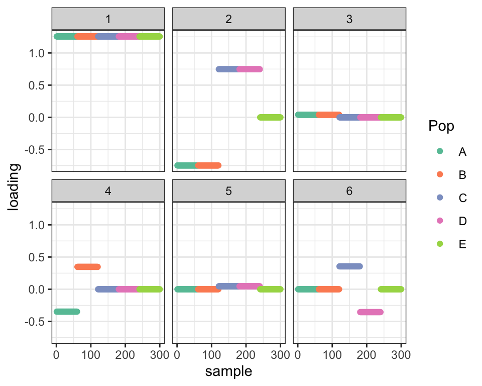
Namely, I’m initializing the tree by using a mixture of point masses at -1, 0, and +1, with the point mass at zero corresponding to either zero participation in the corresponding subtree or a 50-50 admixture. For example, admixture proportions of \(1/2\), \(1/3\), and \(1/6\) would give a 50-50 admixture for the top split (between Populations \(A/B\) and Populations \(C/D\)), so that we’d expect the loading for Population \(E\) to be zero. With a 60-25-15 admixture, we’d instead like to see a loading of \(1/5\).

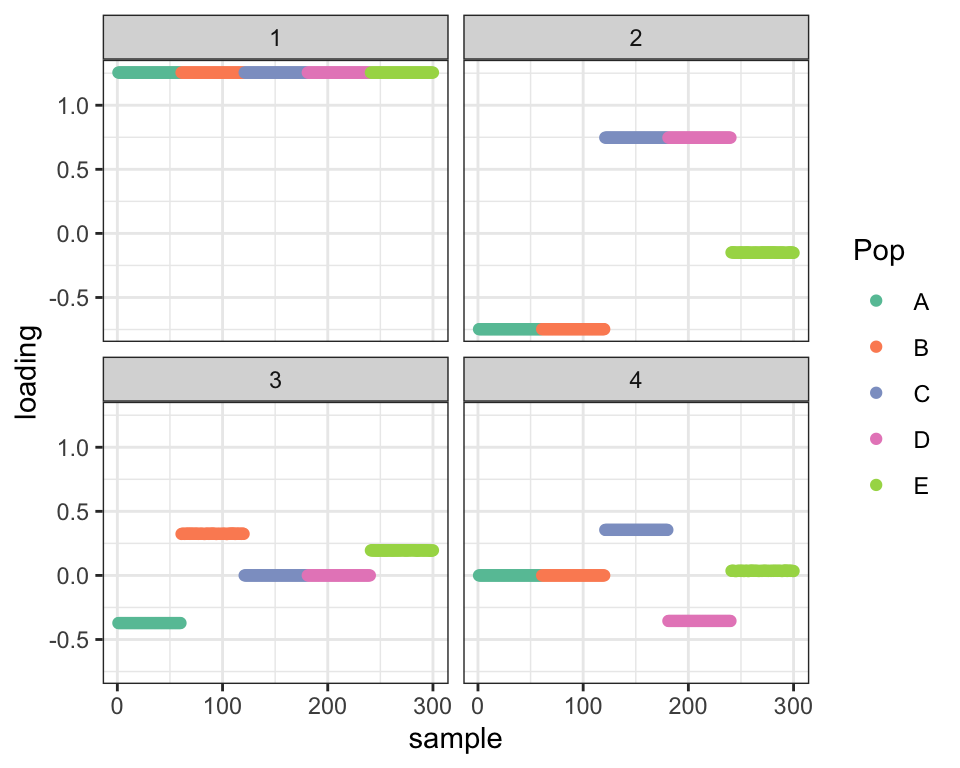
After initializing the tree, I’ll re-fit using a more flexible mixture of point masses at -1 and +1 and then a uniform component on \([-0.9, 0.9]\). I don’t want to allow the uniform component to span the entire interval between -1 and +1: the optimization seems to be a little easier when the difference between the pointmass and the uniform component is exaggerated. This should be fine for all but the worst of cases (i.e., very small admixture proportions for the top split).

set.seed(666)

n_per_pop <- 60
p <- 10000

a <- rnorm(p)
b <- rnorm(p)
c <- rnorm(p)
d <- rnorm(p, sd = 0.5)
e <- rnorm(p, sd = 0.5)
f <- rnorm(p, sd = 0.5)
g <- rnorm(p, sd = 0.5)

popA <- c(rep(1, n_per_pop), rep(0, 4 * n_per_pop))
popB <- c(rep(0, n_per_pop), rep(1, n_per_pop), rep(0, 3 * n_per_pop))
popC <- c(rep(0, 2 * n_per_pop), rep(1, n_per_pop), rep(0, 2 * n_per_pop))
popD <- c(rep(0, 3 * n_per_pop), rep(1, n_per_pop), rep(0, n_per_pop))
popE <- c(rep(0, 4 * n_per_pop), rep(1, n_per_pop))

E.factor <- 0.60 * (a + b + e) + 0.25 * (a + c + f) + 0.15 * (a + c + g)

Y <- cbind(popA, popB, popC, popD, popE) %*% 
  rbind(a + b + d, a + b + e, a + c + f, a + c + g, E.factor)
Y <- Y + rnorm(5 * n_per_pop * p, sd = 0.1)

plot_dr <- function(dr) {
  sd <- sqrt(dr$prior_s2)
  L <- dr$EL
  LDsqrt <- L %*% diag(sd)
  K <- ncol(LDsqrt)
  plot_loadings(LDsqrt[,1:K], rep(c("A", "B", "C", "D", "E"), each = n_per_pop)) +
    scale_color_brewer(palette="Set2")
}

tree.fn = function(x, s, g_init, fix_g, output, ...) {
  if (is.null(g_init)) {
    g_init <- ashr::unimix(rep(1/3, 3), c(-1, 0, 1), c(-1, 0, 1))
  }

  return(flashier:::ebnm.nowarn(x = x,
                                s = s,
                                g_init = g_init,
                                fix_g = fix_g,
                                output = output,
                                prior_family = "ash",
                                prior = c(10, 1, 10),
                                ...))
}

prior.tree = function(...) {
  return(as.prior(sign = 0, ebnm.fn = function(x, s, g_init, fix_g, output) {
    tree.fn(x, s, g_init, fix_g, output, ...)
  }))
}

flextree.fn = function(x, s, g_init, fix_g, output, ...) {
  if (is.null(g_init)) {
    g_init <- ashr::unimix(rep(1/3, 3), c(-1, -0.9, 1), c(-1, 0.9, 1))
  }

  return(flashier:::ebnm.nowarn(x = x,
                                s = s,
                                g_init = g_init,
                                fix_g = fix_g,
                                output = output,
                                prior_family = "ash",
                                prior = c(10, 1, 10),
                                ...))
}

prior.flextree = function(...) {
  return(as.prior(sign = 0, ebnm.fn = function(x, s, g_init, fix_g, output) {
    flextree.fn(x, s, g_init, fix_g, output, ...)
  }))
}

Here’s what the initial tree looks like with the three-pointmass priors. I added extra “mean” factors for Populations \(A/B\) and Populations \(C/D\) (Factors 3 and 5 below), basically to subtract out the contribution from Population \(E\) before splitting. I’ll be able to remove those factors when I use the more relaxed priors.

ones <- matrix(1, nrow = nrow(Y), ncol = 1)
ls.soln <- t(solve(crossprod(ones), crossprod(ones, Y)))

fl <- flash.init(Y) %>%
  flash.set.verbose(0) %>%
  flash.init.factors(EF = list(ones, ls.soln), 
                     prior.family = c(prior.tree(), prior.normal())) %>%
  flash.fix.loadings(kset = 1, mode = 1L) %>%
  flash.backfit() %>%
  flash.add.greedy(prior.family = c(prior.tree(), prior.normal())) %>%
  flash.backfit()

set1 <- (fl$flash.fit$EF[[1]][, 2] < -0.9)
set2 <- (fl$flash.fit$EF[[1]][, 2] > 0.9)
set3 <- !set1 & !set2 # admixed individuals

# Add a mean factor for Populations A/B.

next.factor <- matrix(1L * set1, ncol = 1)
ls.soln <- t(solve(crossprod(next.factor), crossprod(next.factor, Y)))

fl2 <- fl %>%
  flash.init.factors(EF = list(next.factor, ls.soln),
                     prior.family = c(prior.tree(), prior.normal())) %>%
  flash.fix.loadings(kset = 3, mode = 1L) %>%
  flash.backfit(3)

# Split A/B.

next.factor <- matrix(sample(c(-1, 1), size = nrow(Y), replace = TRUE) * set1, ncol = 1)
ls.soln <- t(solve(crossprod(next.factor), crossprod(next.factor, Y)))

fl2 <- fl2 %>%
  flash.init.factors(EF = list(next.factor, ls.soln),
                     prior.family = c(prior.tree(), prior.normal())) %>%
  flash.fix.loadings(kset = 4, mode = 1L, is.fixed = set2 | set3) %>%
  flash.backfit(4)

# Add a mean factor for Populations C/D.

next.factor <- matrix(1L * set2, ncol = 1)
ls.soln <- t(solve(crossprod(next.factor), crossprod(next.factor, Y)))

fl2 <- fl2 %>%
  flash.init.factors(EF = list(next.factor, ls.soln),
                     prior.family = c(prior.tree(), prior.normal())) %>%
  flash.fix.loadings(kset = 5, mode = 1L) %>%
  flash.backfit(5)

# Split C/D.

next.factor <- matrix(sample(c(-1, 1), size = nrow(Y), replace = TRUE) * set2, ncol = 1)
ls.soln <- t(solve(crossprod(next.factor), crossprod(next.factor, Y)))

fl2 <- fl2 %>%
  flash.init.factors(EF = list(next.factor, ls.soln),
                     prior.family = c(prior.tree(), prior.normal())) %>%
  flash.fix.loadings(kset = 6, mode = 1L, is.fixed = set1 | set3) %>%
  flash.backfit(6)

plot_dr(init_from_flash(fl2))

Here’s what the fit looks like after relaxation.

# Remove the redundant "mean" factors.
fl3 <- fl2 %>%
  flash.fix.loadings(kset = 4, mode = 1L, is.fixed = set2) %>%
  flash.fix.loadings(kset = 6, mode = 1L, is.fixed = set1) %>%
  flash.remove.factors(c(3, 5)) %>%
  flash.backfit()

# Relax the priors.
for (k in 1:4) {
  fl3$flash.fit$ebnm.fn[[k]][[1]] <- flextree.fn
}

# Refit.
fl3 <- fl3 %>% flash.backfit(warmstart = FALSE)
  
plot_dr(init_from_flash(fl3))

This looks pretty good. For Population \(E\), we want to see loadings of \(0.4 - 0.6 = -0.2\) for the top split (Factor 2), \(0.6\) for Factor 3, and \(0.25 - 0.15 = 0.1\) for Factor 4. And that’s pretty much what we see (with the exception that there’s noticeable shrinkage for Factor 3):

LL <- colMeans(fl3$flash.fit$EF[[1]][241:300, ])
names(LL) <- paste("Factor", 1:4)
round(LL, 2)

#> Factor 1 Factor 2 Factor 3 Factor 4 
#>     1.00    -0.20     0.52     0.10

Session information

sessionInfo()

#> R version 3.5.3 (2019-03-11)
#> Platform: x86_64-apple-darwin15.6.0 (64-bit)
#> Running under: macOS Mojave 10.14.6
#> 
#> Matrix products: default
#> BLAS: /Library/Frameworks/R.framework/Versions/3.5/Resources/lib/libRblas.0.dylib
#> LAPACK: /Library/Frameworks/R.framework/Versions/3.5/Resources/lib/libRlapack.dylib
#> 
#> locale:
#> [1] en_US.UTF-8/en_US.UTF-8/en_US.UTF-8/C/en_US.UTF-8/en_US.UTF-8
#> 
#> attached base packages:
#> [1] stats     graphics  grDevices utils     datasets  methods   base     
#> 
#> other attached packages:
#>  [1] forcats_0.4.0     stringr_1.4.0     dplyr_0.8.0.1    
#>  [4] purrr_0.3.2       readr_1.3.1       tidyr_0.8.3      
#>  [7] tibble_2.1.1      ggplot2_3.2.0     tidyverse_1.2.1  
#> [10] drift.alpha_0.0.9 flashier_0.2.5   
#> 
#> loaded via a namespace (and not attached):
#>  [1] Rcpp_1.0.4.6       lubridate_1.7.4    invgamma_1.1      
#>  [4] lattice_0.20-38    assertthat_0.2.1   rprojroot_1.3-2   
#>  [7] digest_0.6.18      truncnorm_1.0-8    R6_2.4.0          
#> [10] cellranger_1.1.0   plyr_1.8.4         backports_1.1.3   
#> [13] evaluate_0.13      httr_1.4.0         pillar_1.3.1      
#> [16] rlang_0.4.2        lazyeval_0.2.2     readxl_1.3.1      
#> [19] rstudioapi_0.10    ebnm_0.1-21        irlba_2.3.3       
#> [22] whisker_0.3-2      Matrix_1.2-15      rmarkdown_1.12    
#> [25] labeling_0.3       munsell_0.5.0      mixsqp_0.3-40     
#> [28] broom_0.5.1        compiler_3.5.3     modelr_0.1.5      
#> [31] xfun_0.6           pkgconfig_2.0.2    SQUAREM_2017.10-1 
#> [34] htmltools_0.3.6    tidyselect_0.2.5   workflowr_1.2.0   
#> [37] withr_2.1.2        crayon_1.3.4       grid_3.5.3        
#> [40] nlme_3.1-137       jsonlite_1.6       gtable_0.3.0      
#> [43] git2r_0.25.2       magrittr_1.5       scales_1.0.0      
#> [46] cli_1.1.0          stringi_1.4.3      reshape2_1.4.3    
#> [49] fs_1.2.7           xml2_1.2.0         generics_0.0.2    
#> [52] RColorBrewer_1.1-2 tools_3.5.3        glue_1.3.1        
#> [55] hms_0.4.2          parallel_3.5.3     yaml_2.2.0        
#> [58] colorspace_1.4-1   ashr_2.2-51        rvest_0.3.4       
#> [61] knitr_1.22         haven_2.1.1