Revisiting prior families for trees: Part VI
Jason Willwerscheid
7/22/2020
Last updated: 2020-08-01
Checks: 6 0
Knit directory: drift-workflow/analysis/
This reproducible R Markdown analysis was created with workflowr (version 1.2.0). The Report tab describes the reproducibility checks that were applied when the results were created. The Past versions tab lists the development history.
Great! Since the R Markdown file has been committed to the Git repository, you know the exact version of the code that produced these results.
Great job! The global environment was empty. Objects defined in the global environment can affect the analysis in your R Markdown file in unknown ways. For reproduciblity it’s best to always run the code in an empty environment.
The command set.seed(20190211) was run prior to running the code in the R Markdown file. Setting a seed ensures that any results that rely on randomness, e.g. subsampling or permutations, are reproducible.
Great job! Recording the operating system, R version, and package versions is critical for reproducibility.
Nice! There were no cached chunks for this analysis, so you can be confident that you successfully produced the results during this run.
Great! You are using Git for version control. Tracking code development and connecting the code version to the results is critical for reproducibility. The version displayed above was the version of the Git repository at the time these results were generated.
Note that you need to be careful to ensure that all relevant files for the analysis have been committed to Git prior to generating the results (you can use wflow_publish or wflow_git_commit). workflowr only checks the R Markdown file, but you know if there are other scripts or data files that it depends on. Below is the status of the Git repository when the results were generated:
Ignored files:
    Ignored:    .DS_Store
    Ignored:    .Rhistory
    Ignored:    .Rproj.user/
    Ignored:    docs/.DS_Store
    Ignored:    docs/assets/.DS_Store
    Ignored:    output/

Untracked files:
    Untracked:  analysis/extrapolate3.Rmd
    Untracked:  analysis/extrapolate4.Rmd

Unstaged changes:
    Modified:   drift-workflow.Rproj
Note that any generated files, e.g. HTML, png, CSS, etc., are not included in this status report because it is ok for generated content to have uncommitted changes.
These are the previous versions of the R Markdown and HTML files. If you’ve configured a remote Git repository (see ?wflow_git_remote), click on the hyperlinks in the table below to view them.
| File | Version | Author | Date | Message |
|---|---|---|---|---|
| Rmd | fa11a54 | Jason Willwerscheid | 2020-08-01 | workflowr::wflow_publish(“analysis/pm1_priors6.Rmd”) |
| html | 89c4727 | Jason Willwerscheid | 2020-08-01 | Build site. |
| Rmd | aa25c3e | Jason Willwerscheid | 2020-08-01 | workflowr::wflow_publish(“analysis/pm1_priors6.Rmd”) |
suppressMessages({
  library(flashier)
  library(drift.alpha)
  library(tidyverse)
})
I again simulate a tree with 8 populations, but I remove the admixed populations. I use identical branch lengths to illustrate the problems that can arise as a result.
set.seed(666)

p <- 10000
resid_sd <- 0.1

# Define tree by mean branch length at each depth:
branch_means <- rep(1, 4)
branch_sds <- rep(0, 4)
depth <- length(branch_means)
npop_pure <- 2^(depth - 1)

# Define admixtures by admixture proportions:
admix_pops <- matrix(nrow = 0, ncol = 0)
npop_admix <- ncol(admix_pops)

npop <- npop_pure + npop_admix

n <- sample(50, npop, replace = TRUE)
K <- 2^depth - 1

FF <- matrix(nrow = p, ncol = K)
k <- 1
for (d in 1:depth) {
  for (i in 1:(2^(d - 1))) {
    FF[, k] <- rnorm(p, sd = branch_means[d] + rnorm(1, sd = branch_sds[d]))
    k <- k + 1
  }
}

tree_mat <- matrix(0, nrow = npop_pure, ncol = K)
k <- 1
for (d in 1:depth) {
  size <- 2^(depth - d)
  for (i in 1:(2^(d - 1))) {
    tree_mat[((i - 1) * size + 1):(i * size), k] <- 1
    k <- k + 1
  }
}

pop_means <- FF %*% t(tree_mat)
if (npop_admix > 0) {
  pop_means <- cbind(pop_means, pop_means %*% admix_pops)
}

Y <- NULL
for (i in 1:npop) {
  Y <- rbind(Y, matrix(pop_means[, i], nrow = n[i], ncol = p, byrow = TRUE))
}
Y <- Y + rnorm(n * p, sd = resid_sd)

plot_dr <- function(dr) {
  sd <- sqrt(dr$prior_s2)
  L <- dr$EL
  LDsqrt <- L %*% diag(sd)
  K <- ncol(LDsqrt)
  plot_loadings(LDsqrt[,1:K], rep(letters[1:npop], n)) +
    scale_color_brewer(palette="Set3")
}

tree.fn = function(x, s, g_init, fix_g, output, ...) {
  if (is.null(g_init)) {
    g_init <- ashr::unimix(rep(1/3, 3), c(-1, 0, 1), c(-1, 0, 1))
  }

  return(flashier:::ebnm.nowarn(x = x,
                                s = s,
                                g_init = g_init,
                                fix_g = fix_g,
                                output = output,
                                prior_family = "ash",
                                prior = c(10, 1, 10),
                                ...))
}

prior.tree = function(...) {
  return(as.prior(sign = 0, ebnm.fn = function(x, s, g_init, fix_g, output) {
    tree.fn(x, s, g_init, fix_g, output, ...)
  }))
}

flextree.fn = function(a = 0, b = 1) {
  return(function(x, s, g_init, fix_g, output, ...) {
  if (is.null(g_init)) {
    g_init <- ashr::unimix(rep(1/5, 5), c(-1, 0, 1, -b, a), c(-1, 0, 1, -a, b))
  }

  return(flashier:::ebnm.nowarn(x = x,
                                s = s,
                                g_init = g_init,
                                fix_g = fix_g,
                                output = output,
                                prior_family = "ash",
                                prior = c(10, 10, 10, 1, 1),
                                ...))
  })
}

prior.flextree = function(...) {
  return(as.prior(sign = 0, ebnm.fn = function(x, s, g_init, fix_g, output) {
    flextree.fn(x, s, g_init, fix_g, output, ...)
  }))
}

init.mean.factor <- function(resids, zero.idx) {
  u <- matrix(1, nrow = nrow(resids), ncol = 1)
  u[zero.idx, 1] <- 0
  v <- t(solve(crossprod(u), crossprod(u, resids)))
  return(list(u, v))
}

init.split.factor <- function(resids, zero.idx) {
  svd.res <- svd(resids, nu = 1, nv = 1)
  u <- svd.res$u
  u[zero.idx] <- 0
  u <- matrix(sign(u), ncol = 1)
  v <- t(solve(crossprod(u), crossprod(u, resids)))
  return(list(u, v))
}
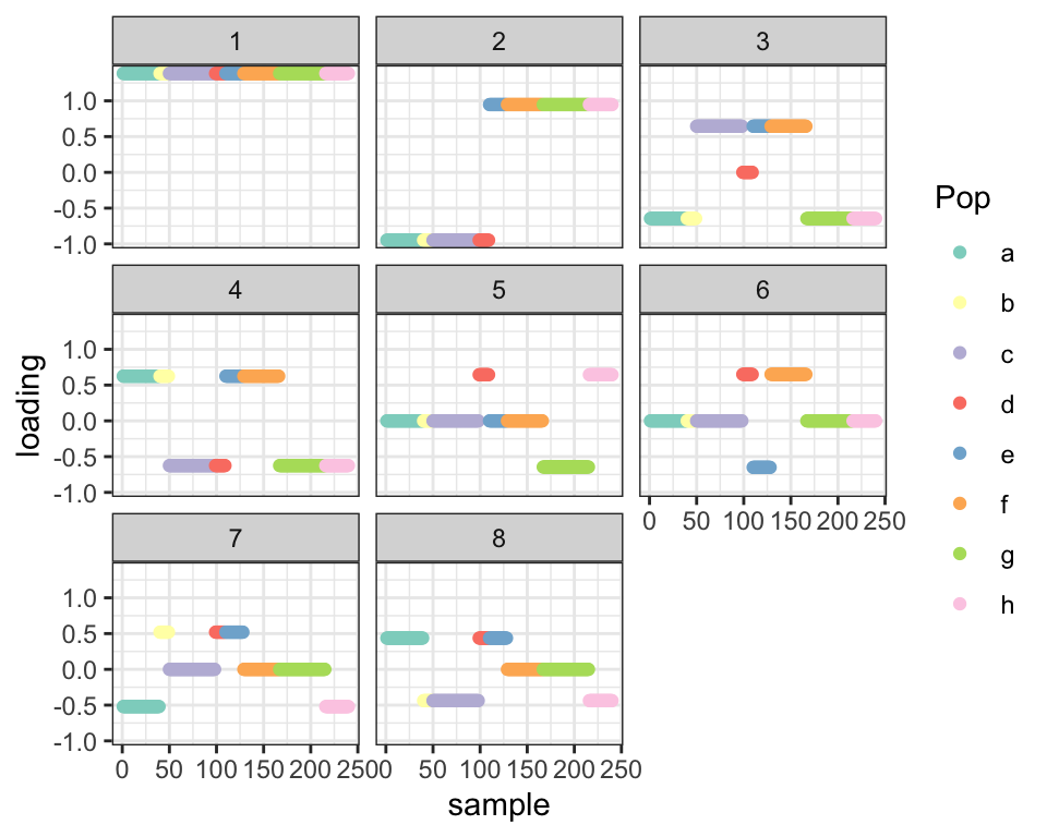
I only show the initialization here (with no relaxation). Factor 2 looks good, but subsequent factors are jumbled.
fl <- flash.init(Y) %>%
  flash.set.verbose(0) %>%
  flash.init.factors(EF = init.mean.factor(Y, NULL),
                     prior.family = c(prior.tree(), prior.normal())) %>%
  flash.fix.loadings(kset = 1, mode = 1L) %>%
  flash.backfit() %>%
  flash.add.greedy(Kmax = npop_pure - 1,
                   prior.family = c(prior.tree(), prior.normal())) %>%
  flash.backfit()

fl2 <- fl

# Partial relaxation.
for (k in 1:fl2$n.factors) {
  fl2$flash.fit$ebnm.fn[[k]][[1]] <- flextree.fn(a = 0, b = 0.9)
}
fl2 <- fl2 %>% flash.backfit(warmstart = FALSE) %>% flash.backfit()

plot_dr(init_from_flash(fl))
| Version | Author | Date |
|---|---|---|
| 89c4727 | Jason Willwerscheid | 2020-08-01 |
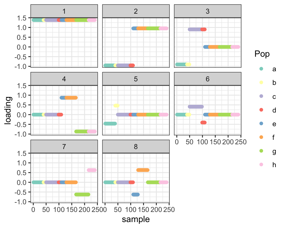
One way to handle this problem is to impose a “hard” tree constraint on the initial fit. By doing so, each factor can be interpreted as a sub-partition of a previous partition, so that a binary tree can be easily reconstructed:
add_split <- function(fl, k) {
  set1 <- (fl$flash.fit$EF[[1]][, k] < -0.9)
  set2 <- (fl$flash.fit$EF[[1]][, k] > 0.9)
  set3 <- !set1 & !set2 # admixed individuals

  n.factors <- fl$n.factors

  fl2 <- fl %>%
    flash.init.factors(EF = init.mean.factor(Y - fitted(fl), set2 | set3),
                       prior.family = c(prior.tree(), prior.normal())) %>%
    flash.fix.loadings(kset = n.factors + 1, mode = 1L) %>%
    flash.backfit(n.factors + 1)

  fl2 <- fl2 %>%
    flash.init.factors(EF = init.split.factor(Y - fitted(fl2), set2 | set3),
                       prior.family = c(prior.tree(), prior.normal())) %>%
    flash.fix.loadings(kset = n.factors + 2, mode = 1L, is.fixed = set2 | set3) %>%
    flash.backfit(n.factors + 2)

  fl2 <- fl2 %>%
    flash.init.factors(EF = init.mean.factor(Y - fitted(fl2), set1 | set3),
                       prior.family = c(prior.tree(), prior.normal())) %>%
    flash.fix.loadings(kset = n.factors + 3, mode = 1L) %>%
    flash.backfit(n.factors + 3)

  fl2 <- fl2 %>%
    flash.init.factors(EF = init.split.factor(Y - fitted(fl2), set1 | set3),
                       prior.family = c(prior.tree(), prior.normal())) %>%
    flash.fix.loadings(kset = n.factors + 4, mode = 1L, is.fixed = set1 | set3) %>%
    flash.backfit(n.factors + 4)

  fl2 <- fl2 %>%
    flash.remove.factors(kset = c(n.factors + 1, n.factors + 3))

  return(fl2)
}

fl3 <- flash.init(Y) %>%
  flash.set.verbose(0) %>%
  flash.init.factors(EF = init.mean.factor(Y, NULL),
                     prior.family = c(prior.tree(), prior.normal())) %>%
  flash.fix.loadings(kset = 1, mode = 1L) %>%
  flash.backfit() %>%
  flash.add.greedy(prior.family = c(prior.tree(), prior.normal())) %>%
  flash.backfit()

fl3 <- fl3 %>% add_split(k = 2)

fl3 <- fl3 %>% add_split(k = 3) %>% add_split(k = 4)

plot_dr(init_from_flash(fl3))
| Version | Author | Date |
|---|---|---|
| 89c4727 | Jason Willwerscheid | 2020-08-01 |
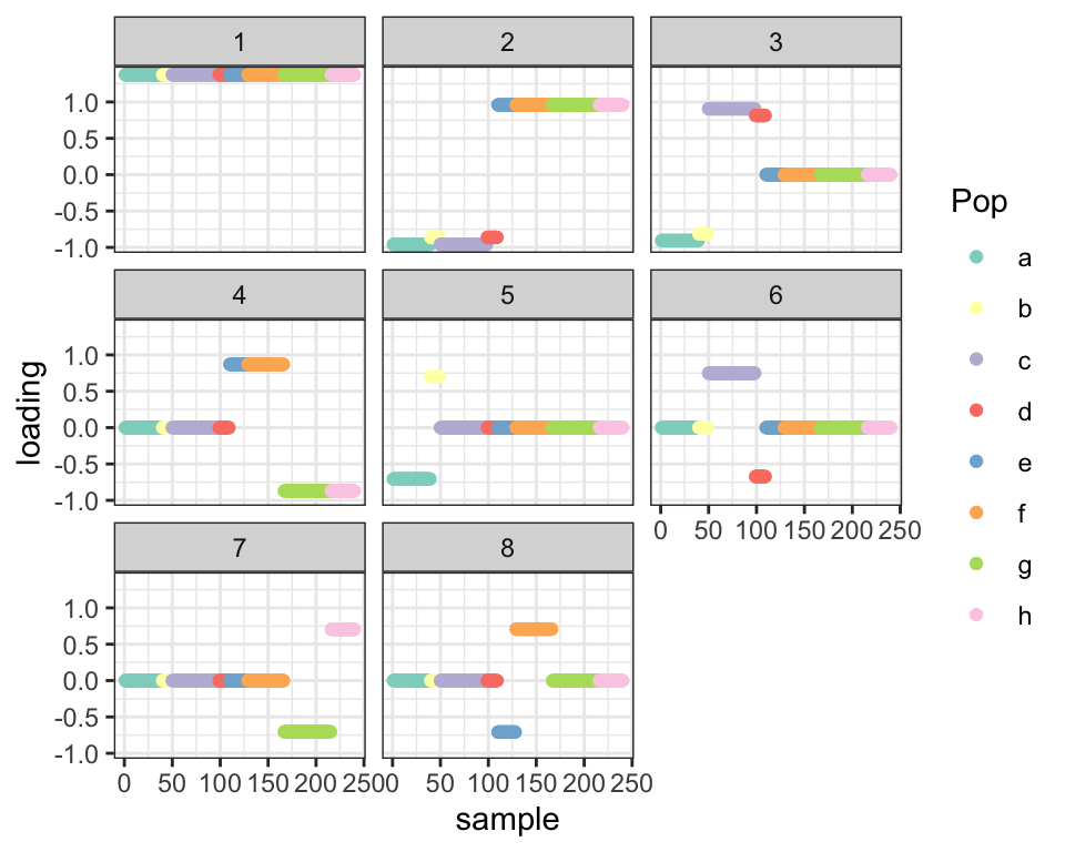
Now I “relax” this fit. I relax the priors and then I unfix all loadings (with the exception of the first factor k = 1). It’s not perfect; in particular, smaller populations have loadings that are not as large as they should be. Still, it’s easy to spot the tree here:
fl4 <- fl3

for (k in 1:fl4$n.factors) {
  fl4$flash.fit$ebnm.fn[[k]][[1]] <- flextree.fn(a = 0, b = 0.9)
}
fl4 <- fl4 %>% flash.backfit(warmstart = FALSE) %>% flash.backfit()

fl5 <- fl4 %>%
  flash.fix.loadings(kset = 3:fl4$n.factors, mode = 1, is.fixed = FALSE) %>%
  flash.backfit()

plot_dr(init_from_flash(fl5))
| Version | Author | Date |
|---|---|---|
| 89c4727 | Jason Willwerscheid | 2020-08-01 |
The second fit has a slightly lower ELBO, which can be explained by a lower KL-divergence for the loadings:
cat("ELBO (without tree constraint):", fl2$elbo,
    "\nELBO (with tree constraint):   ", fl5$elbo,
    "\nKL-div (loadings, no tree):  ", sum(fl2$flash.fit$KL[[1]]),
    "\nKL-div (loadings, with tree):", sum(fl5$flash.fit$KL[[1]]))
#> ELBO (without tree constraint): 2726712
#> ELBO (with tree constraint): 2726650
#> KL-div (loadings, no tree): -1605.171
#> KL-div (loadings, with tree): -2091.872
sessionInfo()#> R version 3.5.3 (2019-03-11)
#> Platform: x86_64-apple-darwin15.6.0 (64-bit)
#> Running under: macOS Mojave 10.14.6
#>
#> Matrix products: default
#> BLAS: /Library/Frameworks/R.framework/Versions/3.5/Resources/lib/libRblas.0.dylib
#> LAPACK: /Library/Frameworks/R.framework/Versions/3.5/Resources/lib/libRlapack.dylib
#>
#> locale:
#> [1] en_US.UTF-8/en_US.UTF-8/en_US.UTF-8/C/en_US.UTF-8/en_US.UTF-8
#>
#> attached base packages:
#> [1] stats graphics grDevices utils datasets methods base
#>
#> other attached packages:
#> [1] forcats_0.4.0 stringr_1.4.0 dplyr_0.8.0.1
#> [4] purrr_0.3.2 readr_1.3.1 tidyr_0.8.3
#> [7] tibble_2.1.1 ggplot2_3.2.0 tidyverse_1.2.1
#> [10] drift.alpha_0.0.9 flashier_0.2.7
#>
#> loaded via a namespace (and not attached):
#> [1] Rcpp_1.0.4.6 lubridate_1.7.4 invgamma_1.1
#> [4] lattice_0.20-38 assertthat_0.2.1 rprojroot_1.3-2
#> [7] digest_0.6.18 truncnorm_1.0-8 R6_2.4.0
#> [10] cellranger_1.1.0 plyr_1.8.4 backports_1.1.3
#> [13] evaluate_0.13 httr_1.4.0 pillar_1.3.1
#> [16] rlang_0.4.2 lazyeval_0.2.2 readxl_1.3.1
#> [19] rstudioapi_0.10 ebnm_0.1-21 irlba_2.3.3
#> [22] whisker_0.3-2 Matrix_1.2-15 rmarkdown_1.12
#> [25] labeling_0.3 munsell_0.5.0 mixsqp_0.3-40
#> [28] broom_0.5.1 compiler_3.5.3 modelr_0.1.5
#> [31] xfun_0.6 pkgconfig_2.0.2 SQUAREM_2017.10-1
#> [34] htmltools_0.3.6 tidyselect_0.2.5 workflowr_1.2.0
#> [37] withr_2.1.2 crayon_1.3.4 grid_3.5.3
#> [40] nlme_3.1-137 jsonlite_1.6 gtable_0.3.0
#> [43] git2r_0.25.2 magrittr_1.5 scales_1.0.0
#> [46] cli_1.1.0 stringi_1.4.3 reshape2_1.4.3
#> [49] fs_1.2.7 xml2_1.2.0 generics_0.0.2
#> [52] RColorBrewer_1.1-2 tools_3.5.3 glue_1.3.1
#> [55] hms_0.4.2 parallel_3.5.3 yaml_2.2.0
#> [58] colorspace_1.4-1 ashr_2.2-51 rvest_0.3.4
#> [61] knitr_1.22 haven_2.1.1