Revisiting prior families for trees: Part XII
Jason Willwerscheid
7/22/2020
Last updated: 2020-09-09
Checks: 6 0
Knit directory: drift-workflow/analysis/
This reproducible R Markdown analysis was created with workflowr (version 1.2.0). The Report tab describes the reproducibility checks that were applied when the results were created. The Past versions tab lists the development history.
Great! Since the R Markdown file has been committed to the Git repository, you know the exact version of the code that produced these results.
Great job! The global environment was empty. Objects defined in the global environment can affect the analysis in your R Markdown file in unknown ways. For reproduciblity it’s best to always run the code in an empty environment.
The command set.seed(20190211) was run prior to running the code in the R Markdown file. Setting a seed ensures that any results that rely on randomness, e.g. subsampling or permutations, are reproducible.
Great job! Recording the operating system, R version, and package versions is critical for reproducibility.
Nice! There were no cached chunks for this analysis, so you can be confident that you successfully produced the results during this run.
Great! You are using Git for version control. Tracking code development and connecting the code version to the results is critical for reproducibility. The version displayed above was the version of the Git repository at the time these results were generated.
Note that you need to be careful to ensure that all relevant files for the analysis have been committed to Git prior to generating the results (you can use wflow_publish or wflow_git_commit). workflowr only checks the R Markdown file, but you know if there are other scripts or data files that it depends on. Below is the status of the Git repository when the results were generated:
Ignored files:
    Ignored:    .DS_Store
    Ignored:    .Rhistory
    Ignored:    .Rproj.user/
    Ignored:    docs/.DS_Store
    Ignored:    docs/assets/.DS_Store
    Ignored:    output/

Untracked files:
    Untracked:  analysis/extrapolate3.Rmd
    Untracked:  analysis/extrapolate4.Rmd
    Untracked:  analysis/pm1_priors_tmp.Rmd

Unstaged changes:
    Modified:   analysis/tree_literature.Rmd
    Modified:   drift-workflow.Rproj
Note that any generated files, e.g. HTML, png, CSS, etc., are not included in this status report because it is ok for generated content to have uncommitted changes.
These are the previous versions of the R Markdown and HTML files. If you’ve configured a remote Git repository (see ?wflow_git_remote), click on the hyperlinks in the table below to view them.
| File | Version | Author | Date | Message |
|---|---|---|---|---|
| Rmd | 7475dd4 | Jason Willwerscheid | 2020-09-09 | wflow_publish(“analysis/pm1_priors12.Rmd”) |
| html | 33d694d | Jason Willwerscheid | 2020-09-09 | Build site. |
| Rmd | 29e148e | Jason Willwerscheid | 2020-09-09 | wflow_publish(“analysis/pm1_priors12.Rmd”) |
| html | ae183d9 | Jason Willwerscheid | 2020-09-05 | Build site. |
| Rmd | 109b2d7 | Jason Willwerscheid | 2020-09-05 | wflow_publish(“analysis/pm1_priors12.Rmd”) |
suppressMessages({
  library(flashier)
  library(drift.alpha)
  library(tidyverse)
})
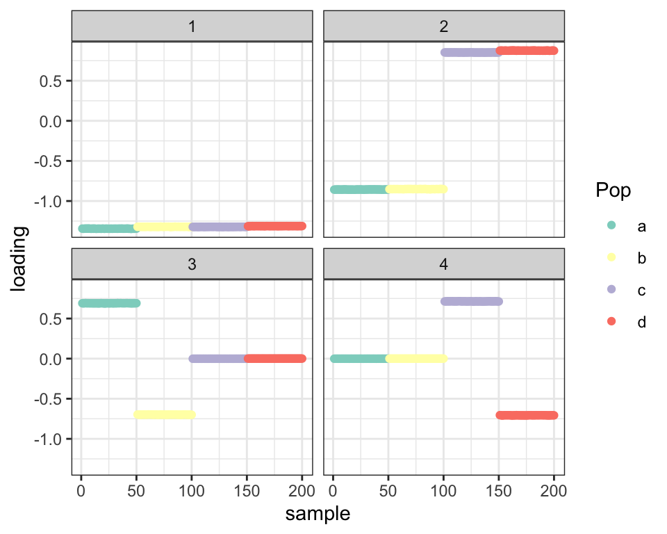
Note that simply running greedy flash on the covariance matrix for the balanced tree with four populations of equal sizes gives us the solution we want.
sim_tree <- function(n_range,
                     p = 10000,
                     branch_means,
                     branch_sds,
                     resid_sd = 0.1,
                     admix_pops = NULL,
                     outgroup = FALSE,
                     seed = 666) {
  set.seed(seed)

  depth <- length(branch_means)
  npop_pure <- 2^(depth - 1)

  if (is.null(admix_pops)) {
    admix_pops <- matrix(nrow = 0, ncol = 0)
  }
  npop_admix <- ncol(admix_pops)

  npop <- npop_pure + npop_admix + outgroup

  if (length(n_range) == 1) {
    n <- rep(n_range, npop)
  } else {
    n <- sample(30:100, npop, replace = TRUE)
  }
  K <- 2^depth - 1

  FF <- matrix(nrow = p, ncol = K)
  k <- 1
  for (d in 1:depth) {
    for (i in 1:(2^(d - 1))) {
      FF[, k] <- rnorm(p, sd = branch_means[d] + rnorm(1, sd = branch_sds[d]))
      k <- k + 1
    }
  }

  tree_mat <- matrix(0, nrow = npop_pure, ncol = K)
  k <- 1
  for (d in 1:depth) {
    size <- 2^(depth - d)
    for (i in 1:(2^(d - 1))) {
      tree_mat[((i - 1) * size + 1):(i * size), k] <- 1
      k <- k + 1
    }
  }

  pop_means <- FF %*% t(tree_mat)
  if (npop_admix > 0) {
    pop_means <- cbind(pop_means, pop_means %*% admix_pops)
  }
  if (outgroup) {
    pop_means <- cbind(pop_means, rnorm(p, mean = 0, sd = sqrt(sum(branch_sds^2))))
  }

  Y <- NULL
  for (i in 1:npop) {
    Y <- rbind(Y, matrix(pop_means[, i], nrow = n[i], ncol = p, byrow = TRUE))
  }
  Y <- Y + rnorm(sum(n) * p, sd = resid_sd)

  plot_fl <- function(fl, mode = 1) {
    LDsqrt <- fl$loadings.pm[[mode]] %*% diag(sqrt(fl$loadings.scale))
    K <- ncol(LDsqrt)
    plot_loadings(LDsqrt[,1:K], rep(letters[1:npop], n)) +
      scale_color_brewer(palette="Set3")
  }

  return(list(Y = Y, plot_fn = plot_fl))
}

init.mean.factor <- function(resids, zero.idx) {
  u <- matrix(1, nrow = nrow(resids), ncol = 1)
  u[zero.idx, 1] <- 0
  v <- t(solve(crossprod(u), crossprod(u, resids)))
  return(list(u, v))
}

balanced_4pop <- sim_tree(n_range = 50,
                          p = 10000,
                          branch_means = rep(1, 3),
                          branch_sds = rep(0, 3),
                          resid_sd = 0.1)
covmat <- cov(t(balanced_4pop$Y))
I use point-Laplace priors with no backfit here:
fl_g <- flash.init(covmat) %>%
  flash.set.verbose(0) %>%
  flash.add.greedy(Kmax = 4,
                   prior.family = prior.point.laplace())

balanced_4pop$plot_fn(fl_g)
| Version | Author | Date |
|---|---|---|
| ae183d9 | Jason Willwerscheid | 2020-09-05 |
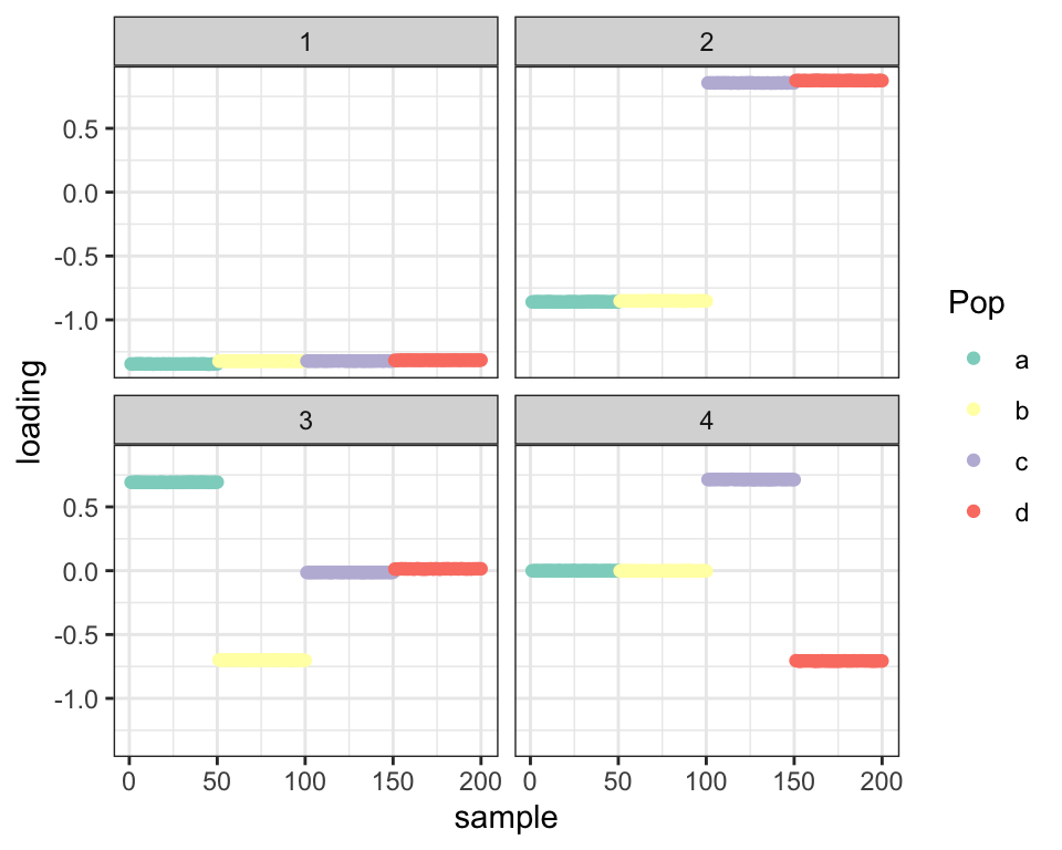
Point-normal priors also work fine:
fl_g2 <- flash.init(covmat) %>%
  flash.set.verbose(0) %>%
  flash.add.greedy(Kmax = 4,
                   prior.family = prior.point.normal())

balanced_4pop$plot_fn(fl_g2)
| Version | Author | Date |
|---|---|---|
| ae183d9 | Jason Willwerscheid | 2020-09-05 |
Assuming that the fit “discovers” the constraint \(L = F\) (and it seems to do so fairly easily), the model here is \[ \text{Cov}(Y) \sim LL' + E \] where \(E\) has the “constant” variance structure \[ E_{ij} \sim N(0, \sigma^2) \]
A better model, however, would fit \[ \text{Cov}(Y) \sim LL' + \sigma_r^2 I + E \] since the expected covariance matrix for \(Y = LF' + E\) when \(F_j \sim N(0, I_p)\) and \(E_{ij} \sim N(0, \sigma_r^2)\) is \(LL' + \sigma_r^2I\). If we put a prior on \(\sigma_r^2 \sim N(0, \sigma_d^2)\), then the model becomes
\[ \text{Cov}(Y) \sim LL' + \tilde{E} \] where \[ \tilde{E}_{ij} \sim N(0, \sigma^2 + \delta_{ij} \sigma_d^2) \] (Note that the MLE for \(\sigma_d^2\) is \(\sigma_r^4\), not \(\sigma_r^2\).) I fit this last model by iterating between 1) estimating \(\sigma_d^2\) and 2) treating \(\sigma_d^2\) as fixed and fitting the flash model using a “noisy” variance structure. I initialize \(\sigma_d^2\) at zero.
fl <- flash.init(covmat) %>%
  flash.set.verbose(0) %>%
  flash.add.greedy(Kmax = 4,
                   prior.family = prior.point.laplace())

n <- nrow(covmat)
diag_S2 <- 0
elbo_diff <- Inf
while (elbo_diff > 0.01) {
  old_elbo <- fl$elbo
  fl <- flash.init(covmat, S = diag(rep(sqrt(diag_S2), n)), var.type = 0) %>%
    flash.set.verbose(0) %>%
    flash.init.factors(EF = fl$flash.fit$EF, EF2 = fl$flash.fit$EF2,
                       prior.family = prior.point.laplace()) %>%
    flash.backfit()
  cat("SD (diagonal):", formatC(sqrt(diag_S2), format = "e", digits = 2),
      " SD (non-diag):", formatC(sqrt(1 / fl$flash.fit$tau[1, 2]), format = "e", digits = 2),
      " ELBO:", fl$elbo, "\n")
  elbo_diff <- fl$elbo - old_elbo

  diag_S2 <- mean(diag(covmat)^2
                  - 2 * diag(covmat) * rowSums(fl$flash.fit$EF[[1]] * fl$flash.fit$EF[[2]])
                  + rowSums(fl$flash.fit$EF2[[1]] * fl$flash.fit$EF2[[2]])
                  - rowSums(fl$flash.fit$EF[[1]]^2 * fl$flash.fit$EF[[2]]^2))
  diag_S2 <- diag_S2 + sum(crossprod(fl$flash.fit$EF[[1]] * fl$flash.fit$EF[[2]])) / n
  diag_S2 <- diag_S2 - 1 / fl$flash.fit$tau[1, 2]
}
#> SD (diagonal): 0.00e+00 SD (non-diag): 7.20e-04 ELBO: 217914.4
#> SD (diagonal): 9.77e-03 SD (non-diag): 9.45e-05 ELBO: 292465.1
#> SD (diagonal): 9.99e-03 SD (non-diag): 9.58e-05 ELBO: 292522.7
#> SD (diagonal): 9.99e-03 SD (non-diag): 9.58e-05 ELBO: 292522.8
#> SD (diagonal): 9.99e-03 SD (non-diag): 9.58e-05 ELBO: 292522.8
balanced_4pop$plot_fn(fl)
| Version | Author | Date |
|---|---|---|
| 33d694d | Jason Willwerscheid | 2020-09-09 |
However, it seems that, as in the previous analysis, some overfitting problems are beginning to rear their heads — adding the diagonal variance term allows the non-diagonal variance to become very small, and as a result few loadings are estimated to be zero. Compare LFSRs for the first fit and this last one:
cat("Nonzero loadings per factor (no diagonal variance term):",
    colSums(fl_g$loadings.lfsr[[1]] < 0.05))
#> Nonzero loadings per factor (no diagonal variance term): 200 200 100 100cat("Nonzero loadings per factor (with diagonal variance):",
colSums(fl$loadings.lfsr[[1]] < 0.05))#> Nonzero loadings per factor (with diagonal variance): 200 200 200 190
sessionInfo()#> R version 3.5.3 (2019-03-11)
#> Platform: x86_64-apple-darwin15.6.0 (64-bit)
#> Running under: macOS Mojave 10.14.6
#>
#> Matrix products: default
#> BLAS: /Library/Frameworks/R.framework/Versions/3.5/Resources/lib/libRblas.0.dylib
#> LAPACK: /Library/Frameworks/R.framework/Versions/3.5/Resources/lib/libRlapack.dylib
#>
#> locale:
#> [1] en_US.UTF-8/en_US.UTF-8/en_US.UTF-8/C/en_US.UTF-8/en_US.UTF-8
#>
#> attached base packages:
#> [1] stats graphics grDevices utils datasets methods base
#>
#> other attached packages:
#> [1] forcats_0.4.0 stringr_1.4.0 dplyr_0.8.0.1
#> [4] purrr_0.3.2 readr_1.3.1 tidyr_0.8.3
#> [7] tibble_2.1.1 ggplot2_3.2.0 tidyverse_1.2.1
#> [10] drift.alpha_0.0.10 flashier_0.2.7
#>
#> loaded via a namespace (and not attached):
#> [1] Rcpp_1.0.4.6 lubridate_1.7.4 invgamma_1.1
#> [4] lattice_0.20-38 assertthat_0.2.1 rprojroot_1.3-2
#> [7] digest_0.6.18 truncnorm_1.0-8 R6_2.4.0
#> [10] cellranger_1.1.0 plyr_1.8.4 backports_1.1.3
#> [13] evaluate_0.13 httr_1.4.0 pillar_1.3.1
#> [16] rlang_0.4.2 lazyeval_0.2.2 readxl_1.3.1
#> [19] rstudioapi_0.10 ebnm_0.1-21 irlba_2.3.3
#> [22] whisker_0.3-2 Matrix_1.2-15 rmarkdown_1.12
#> [25] labeling_0.3 munsell_0.5.0 mixsqp_0.3-40
#> [28] broom_0.5.1 compiler_3.5.3 modelr_0.1.5
#> [31] xfun_0.6 pkgconfig_2.0.2 SQUAREM_2017.10-1
#> [34] htmltools_0.3.6 tidyselect_0.2.5 workflowr_1.2.0
#> [37] withr_2.1.2 crayon_1.3.4 grid_3.5.3
#> [40] nlme_3.1-137 jsonlite_1.6 gtable_0.3.0
#> [43] git2r_0.25.2 magrittr_1.5 scales_1.0.0
#> [46] cli_1.1.0 stringi_1.4.3 reshape2_1.4.3
#> [49] fs_1.2.7 xml2_1.2.0 generics_0.0.2
#> [52] RColorBrewer_1.1-2 tools_3.5.3 glue_1.3.1
#> [55] hms_0.4.2 parallel_3.5.3 yaml_2.2.0
#> [58] colorspace_1.4-1 ashr_2.2-51 rvest_0.3.4
#> [61] knitr_1.22 haven_2.1.1