Simpler tree simulation (bimodal prior)
jhmarcus
2019-05-10
Last updated: 2019-05-20
Checks: 5 1
Knit directory: drift-workflow/analysis/
This reproducible R Markdown analysis was created with workflowr (version 1.2.0). The Report tab describes the reproducibility checks that were applied when the results were created. The Past versions tab lists the development history.
The R Markdown is untracked by Git. To know which version of the R Markdown file created these results, you’ll want to first commit it to the Git repo. If you’re still working on the analysis, you can ignore this warning. When you’re finished, you can run wflow_publish to commit the R Markdown file and build the HTML.
Great job! The global environment was empty. Objects defined in the global environment can affect the analysis in your R Markdown file in unknown ways. For reproduciblity it’s best to always run the code in an empty environment.
The command set.seed(20190211) was run prior to running the code in the R Markdown file. Setting a seed ensures that any results that rely on randomness, e.g. subsampling or permutations, are reproducible.
Great job! Recording the operating system, R version, and package versions is critical for reproducibility.
Nice! There were no cached chunks for this analysis, so you can be confident that you successfully produced the results during this run.
Great! You are using Git for version control. Tracking code development and connecting the code version to the results is critical for reproducibility. The version displayed above was the version of the Git repository at the time these results were generated.
Note that you need to be careful to ensure that all relevant files for the analysis have been committed to Git prior to generating the results (you can use wflow_publish or wflow_git_commit). workflowr only checks the R Markdown file, but you know if there are other scripts or data files that it depends on. Below is the status of the Git repository when the results were generated:
Ignored files:
    Ignored:    .RData
    Ignored:    .Rhistory
    Ignored:    analysis/.Rhistory
    Ignored:    analysis/flash_cache/
    Ignored:    data.tar.gz
    Ignored:    data/datasets/
    Ignored:    data/raw/
    Ignored:    output.tar.gz
    Ignored:    output/

Untracked files:
    Untracked:  analysis/simpler_tree_simulation_bimodal.Rmd
    Untracked:  code/sim.R
    Untracked:  docs/figure/simpler_tree_simulation_bimodal.Rmd/

Unstaged changes:
    Modified:   analysis/index.Rmd
    Modified:   analysis/simpler_tree_simulation.Rmd
    Modified:   code/viz.R
Note that any generated files, e.g. HTML, png, CSS, etc., are not included in this status report because it is ok for generated content to have uncommitted changes.
There are no past versions. Publish this analysis with wflow_publish() to start tracking its development.
In this analysis I simulate data from the same tree as described in Simple Tree Simulation (also see below) but parameterize the simulation as a factor analysis model i.e. simulating under the model we are fitting. I also removed the additional binomial sampling from the allele frequencies at the tips and just directly modeled Gaussian data. 
See code/sim.R for simulation details.
Import
Here I import the some required packages:
library(ggplot2)
library(dplyr)
library(tidyr)
library(ashr)
library(flashier)
source("../code/viz.R")
source("../code/sim.R")
Functions
plot_flash_loadings = function(flash_fit, n_per_pop){

  l_df = as.data.frame(flash_fit$fit$EF[[1]])
  colnames(l_df) = 1:ncol(l_df)
  l_df$ID = 1:nrow(l_df)
  l_df$pop = c(rep("Pop1", n_per_pop), rep("Pop2", n_per_pop),
               rep("Pop3", n_per_pop), rep("Pop4", n_per_pop))

  gath_l_df = l_df %>% gather(K, value, -ID, -pop)

  p1 = ggplot(gath_l_df, aes(x=ID, y=value, color=pop)) +
       geom_point() +
       facet_wrap(K~., scale="free") +
       theme_bw()

  p2 = structure_plot(gath_l_df,
                      colset="Set3",
                      facet_grp="pop",
                      facet_levels=paste0("Pop", 1:4),
                      keep_leg=TRUE,
                      fact_type="nonnegative")

  return(list(p1=p1, p2=p2))

}

my.init.fn <- function(flash, tol, maxiter) {

  EF <- flashier:::init.next.EF(flash, tol, maxiter)

  # Rescale so that L has range 0 to 1.
  l.scale <- max(abs(EF[[1]])) * sign(which.max(abs(EF[[1]])))
  EF[[1]] <- EF[[1]] / l.scale
  EF[[2]] <- EF[[2]] * l.scale

  return(EF)

}
Simulate
Here I simulate a simple tree found here with the below parameter settings:
set.seed(123)
n_per_pop = 20
sigma_e = .5
p = 10000
sim_res = simpler_tree_simulation(n_per_pop, p, sigma_e)
Y = sim_res$Y

l_df = as.data.frame(sim_res$L)
colnames(l_df) = 1:ncol(l_df)
l_df$ID = 1:nrow(l_df)
l_df$pop = c(rep("Pop1", n_per_pop), rep("Pop2", n_per_pop),
             rep("Pop3", n_per_pop), rep("Pop4", n_per_pop))
gath_l_df = l_df %>% gather(K, value, -ID, -pop)
p = ggplot(gath_l_df, aes(x=ID, y=value, color=pop)) +
    geom_point() +
    facet_wrap(K~., scale="free") +
    theme_bw()
p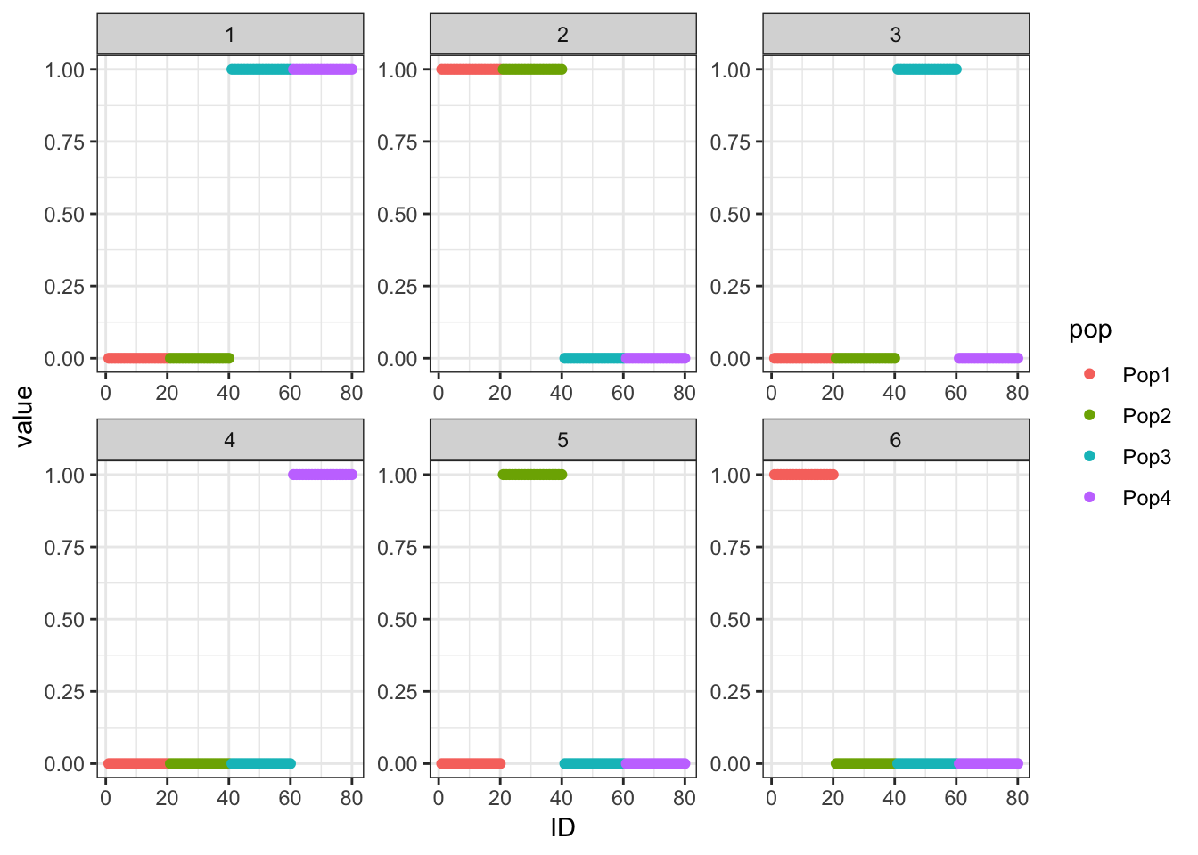
Bimodal prior
Here I specify the grid of the prior
# bimodal g prior list used throughout
m = 20
b = seq(1.0, 0.0, length=m)
a = seq(0.0, 1.0, length=m)
bimodal_g = ashr:::unimix(rep(0, 2*m), c(rep(0, m), b), c(a, rep(1, m)))
Bimodal (Greedy)
flash_fit_g = flashier::flashier(Y,
                                 greedy.Kmax=10,
                                 prior.type=c("nonnegative", "point.normal"),
                                 ash.param=list(fixg=FALSE, g=bimodal_g),
                                 ebnm.param=list(fix_pi0=TRUE, g=list(pi0=0)),
                                 var.type=0,
                                 backfit="none",
                                 init.fn=my.init.fn)
Initializing flash object...
Adding factor 1 to flash object...
Adding factor 2 to flash object...
Adding factor 3 to flash object...
Adding factor 4 to flash object...
Adding factor 5 to flash object...
Adding factor 6 to flash object...
Adding factor 7 to flash object...
Factor doesn't significantly increase objective and won't be added.
Nullchecking 6 factors...
Wrapping up...
Done.Lhat = flash_fit_g$fit$EF[[1]]
p_res = plot_flash_loadings(flash_fit_g, n_per_pop)
print(p_res$p1)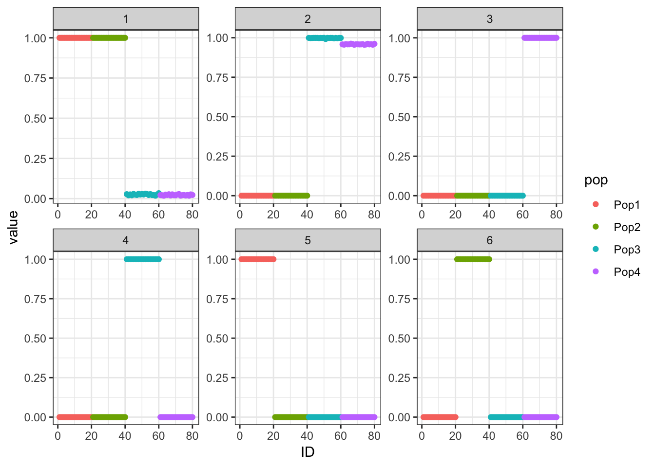
print(p_res$p2)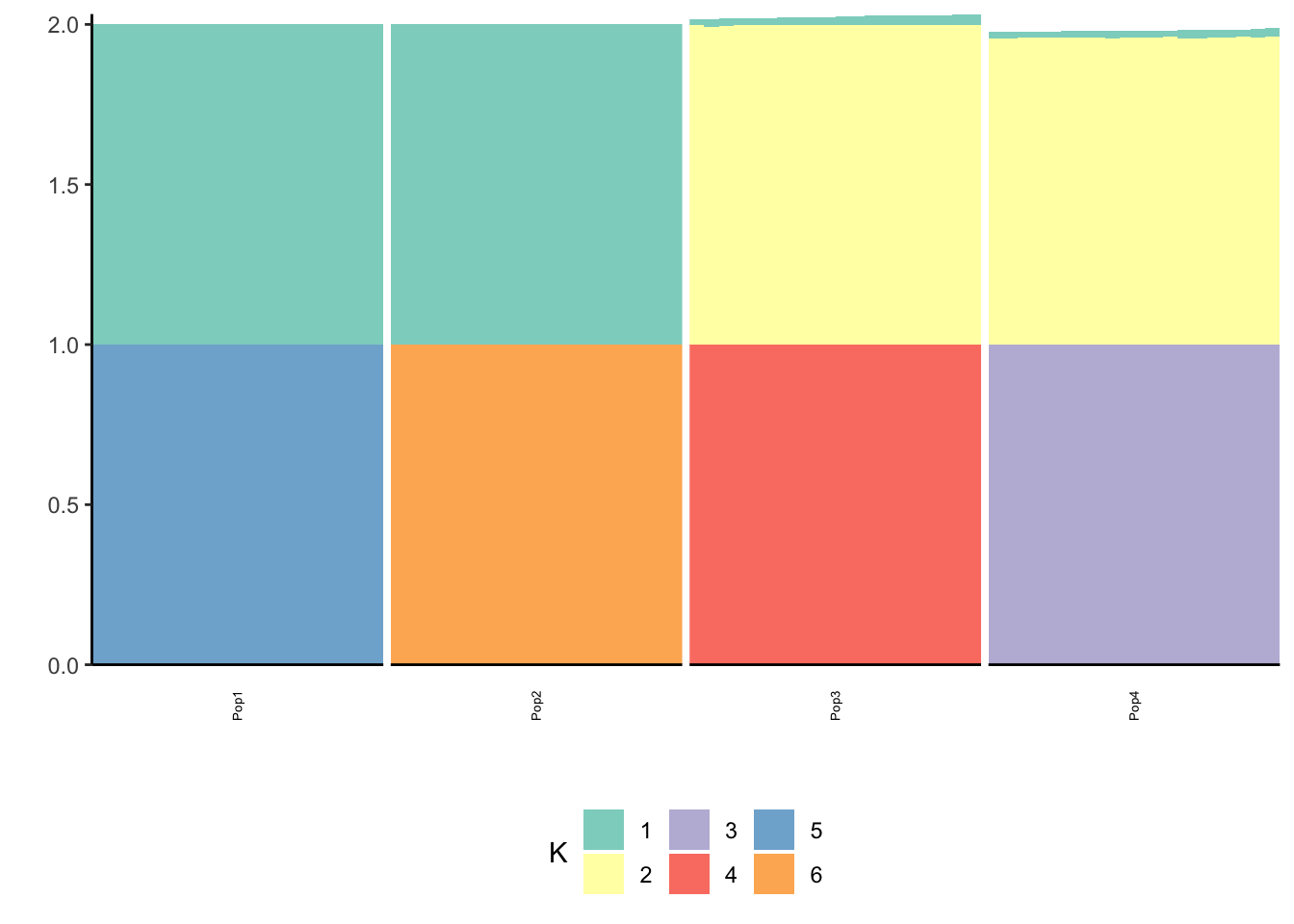
print(plot_covmat(Lhat %*% t(Lhat)))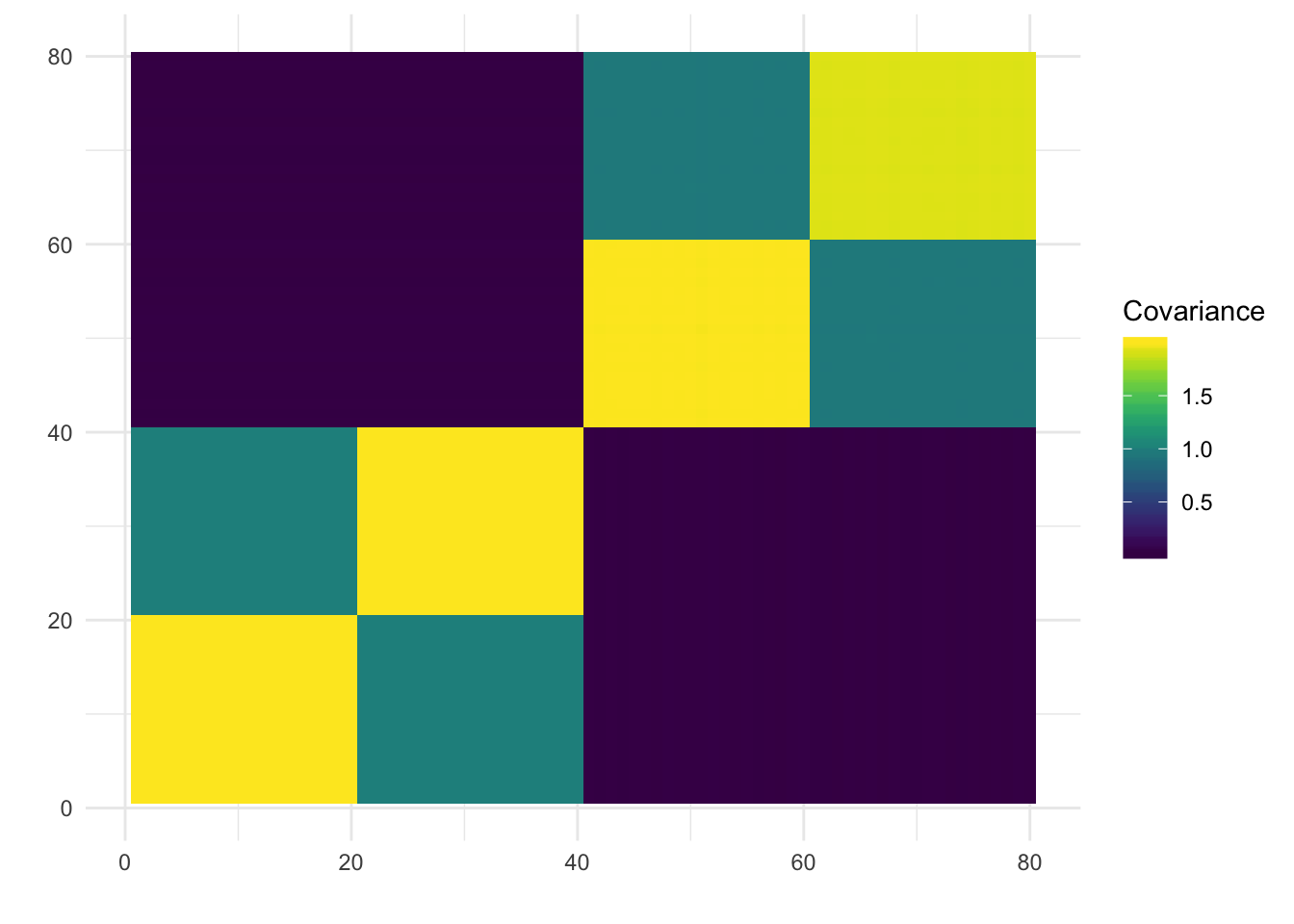
# print sum about the fit
print(paste0("objective =", flash_fit_g$objective))
[1] "objective =-742140.856712264"print(paste0("estimated residual sd =", sqrt(1 / flash_fit_g$fit$tau)))[1] "estimated residual sd =0.537950432041053"print("estimated prior variances (factors)=")[1] "estimated prior variances (factors)="print(sapply(flash_fit_g$fit$g, function(x){1/x[[2]]$a}))[1] 1.4964778 1.5420617 0.5032015 0.4673796 0.4922990 0.4960596Bimodal (montaigne)
flash_fit_bfm = flashier::flashier(Y,
                                  flash.init=flash_fit_g,
                                  greedy.Kmax=10,
                                  prior.type=c("nonnegative", "point.normal"),
                                  ash.param=list(fixg=FALSE, g=bimodal_g),
                                  ebnm.param=list(fix_pi0=TRUE, g=list(pi0=0)),
                                  var.type=0,
                                  backfit="final",
                                  backfit.order="montaigne",
                                  init.fn=my.init.fn)
Initializing flash object...
Adding factor 7 to flash object...
Factor doesn't significantly increase objective and won't be added.
Backfitting 6 factors...
Nullchecking 6 factors...
Wrapping up...
Done.Lhat = flash_fit_bfm$fit$EF[[1]]
p_res = plot_flash_loadings(flash_fit_bfm, n_per_pop)
print(p_res$p1)
print(p_res$p2)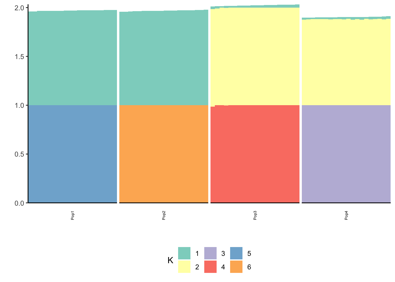
print(plot_covmat(Lhat %*% t(Lhat)))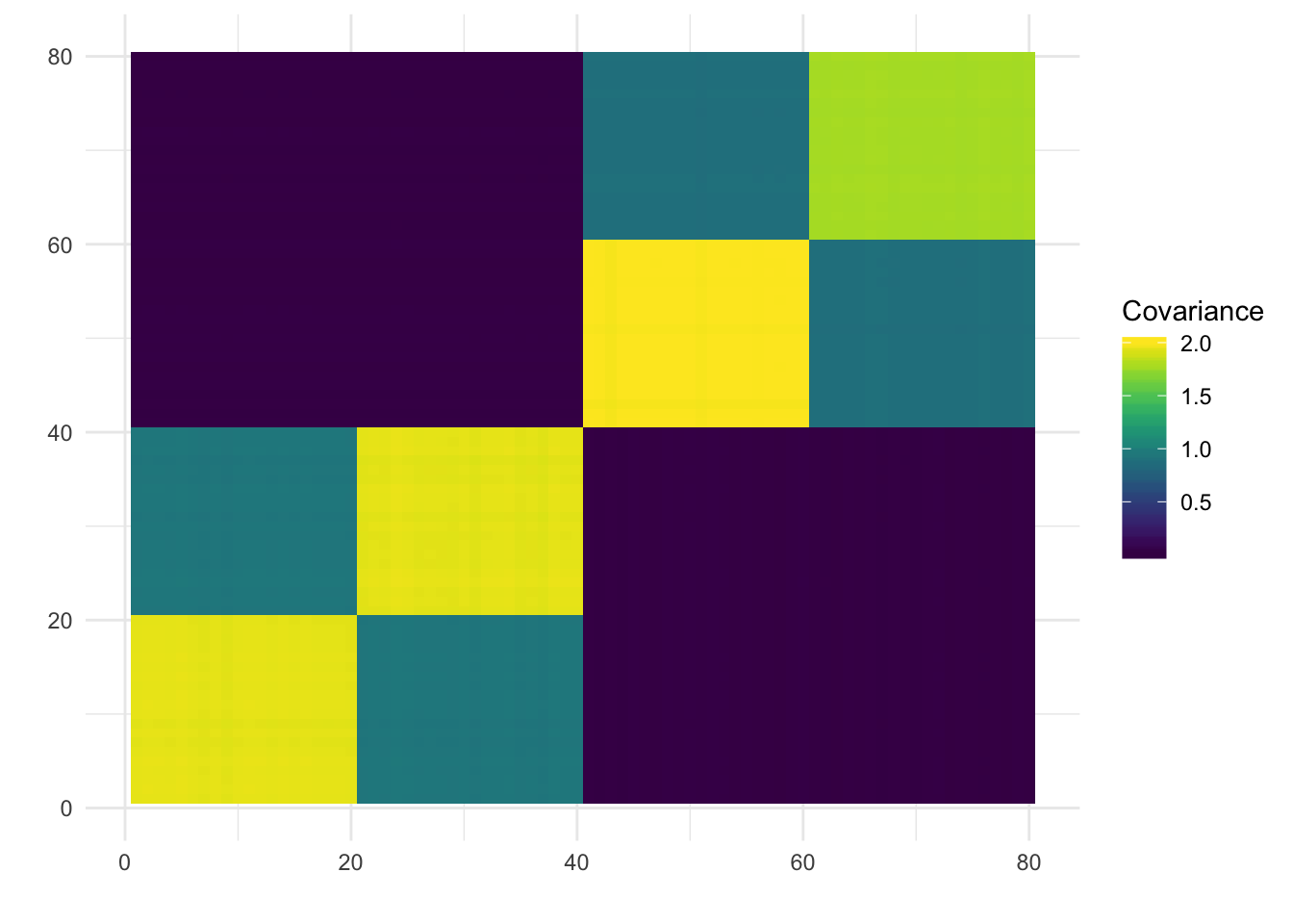
print(paste0("objective =", flash_fit_bfm$objective))[1] "objective =-719400.348180572"print(paste0("estimated residual sd = ", sqrt(1 / flash_fit_bfm$fit$tau)))[1] "estimated residual sd = 0.506714493011869"print("estimated prior variances (factors) =")[1] "estimated prior variances (factors) ="print(sapply(flash_fit_bfm$fit$g, function(x){1/x[[2]]$a}))[1] 1.5270740 1.4668025 0.5425726 0.4853630 0.4947548 0.5048864Bimodal (random)
flash_fit_bfr = flashier::flashier(Y,
                                   flash.init = flash_fit_g,
                                   greedy.Kmax=10,
                                   prior.type=c("nonnegative", "point.normal"),
                                   ash.param=list(fixg=FALSE, g=bimodal_g),
                                   ebnm.param=list(fix_pi0=TRUE, g=list(pi0=0)),
                                   var.type=0,
                                   backfit="final",
                                   backfit.order="random",
                                   init.fn=my.init.fn)
Initializing flash object...
Adding factor 7 to flash object...
Factor doesn't significantly increase objective and won't be added.
Backfitting 6 factors...
An update to factor 6 decreased the objective by 8.149e-09.
Nullchecking 6 factors...
Wrapping up...
Done.Lhat = flash_fit_bfr$fit$EF[[1]]
p_res = plot_flash_loadings(flash_fit_bfr, n_per_pop)
print(p_res$p1)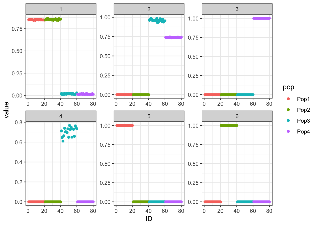
print(p_res$p2)
print(plot_covmat(Lhat %*% t(Lhat)))
print(paste0("objective =", flash_fit_bfr$objective))[1] "objective =-716171.989047966"print(paste0("estimated residual sd =", sqrt(1 / flash_fit_bfr$fit$tau)))[1] "estimated residual sd =0.506525590537778"print("estimated prior variances (factors) =")[1] "estimated prior variances (factors) ="print(sapply(flash_fit_bfr$fit$g, function(x){1/x[[2]]$a}))[1] 1.4371738 1.4875182 0.9721826 0.3895623 0.5614755 0.5306043Bimodal (sequential)
flash_fit_bfs = flashier::flashier(Y,
                                  flash.init = flash_fit_g,
                                  greedy.Kmax=10,
                                  prior.type=c("nonnegative", "point.normal"),
                                  ash.param=list(fixg=FALSE, g=bimodal_g),
                                  ebnm.param=list(fix_pi0=TRUE, g=list(pi0=0)),
                                  var.type=0,
                                  backfit="final",
                                  backfit.order="sequential")
Initializing flash object...
Adding factor 7 to flash object...
Factor doesn't significantly increase objective and won't be added.
Backfitting 6 factors...
Nullchecking 6 factors...
Wrapping up...
Done.Lhat = flash_fit_bfs$fit$EF[[1]]
p_res = plot_flash_loadings(flash_fit_bfs, n_per_pop)
print(p_res$p1)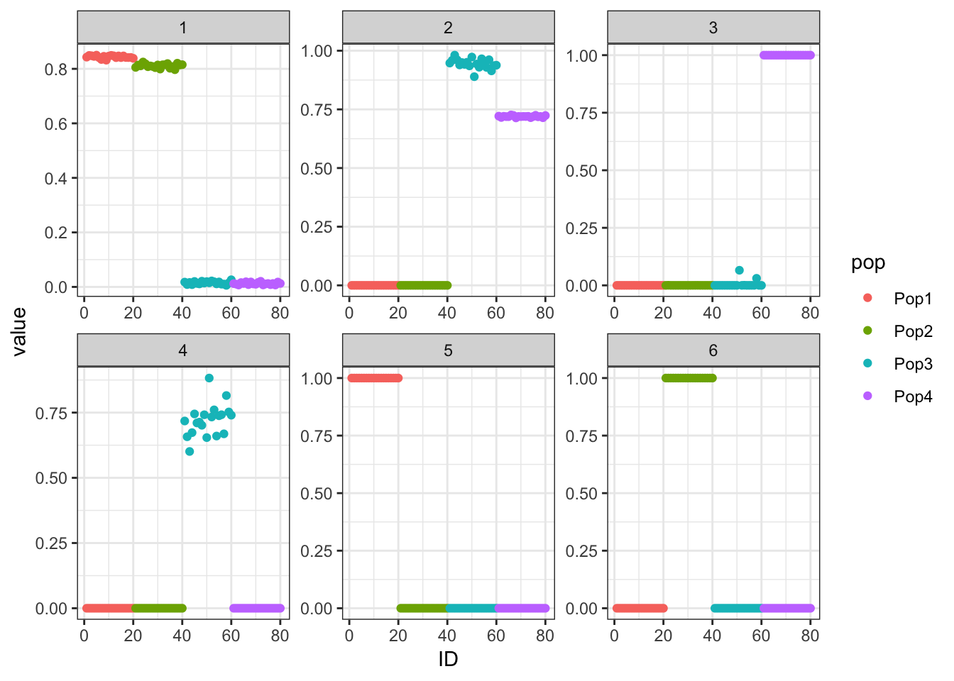
print(p_res$p2)
print(plot_covmat(Lhat %*% t(Lhat)))
print(paste0("objective =", flash_fit_bfs$objective))[1] "objective =-716151.148219496"print(paste0("estimated residual sd =", sqrt(1 / flash_fit_bfs$fit$tau)))[1] "estimated residual sd =0.506379390822608"print("estimated prior variances (factors) =")[1] "estimated prior variances (factors) ="print(sapply(flash_fit_bfs$fit$g, function(x){x[[2]]$a}))[1] 0.6882156 0.6755391 1.0320685 2.4270752 1.9700327 1.6426156Bimodal (dropout)
flash_fit_bfd = flashier::flashier(Y,
                                  flash.init = flash_fit_g,
                                  greedy.Kmax=10,
                                  prior.type=c("nonnegative", "point.normal"),
                                  ash.param=list(fixg=FALSE, g=bimodal_g),
                                  ebnm.param=list(fix_pi0=TRUE, g=list(pi0=0)),
                                  var.type=0,
                                  backfit="final",
                                  backfit.order="dropout")
Initializing flash object...
Adding factor 7 to flash object...
Factor doesn't significantly increase objective and won't be added.
Backfitting 6 factors...
Nullchecking 6 factors...
Wrapping up...
Done.Lhat = flash_fit_bfd$fit$EF[[1]]
p_res = plot_flash_loadings(flash_fit_bfd, n_per_pop)
print(p_res$p1)
print(p_res$p2)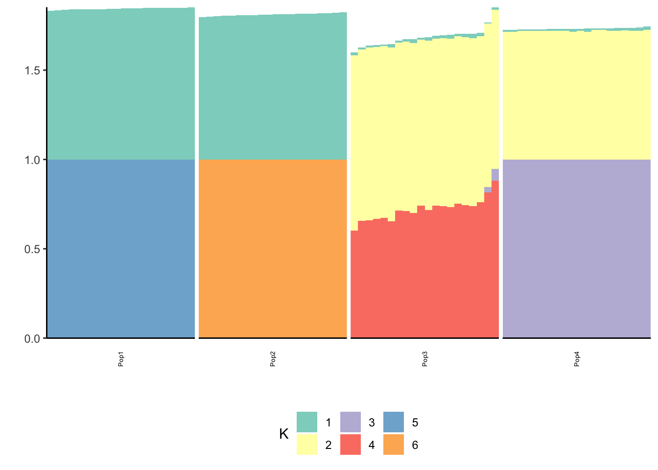
print(plot_covmat(Lhat %*% t(Lhat)))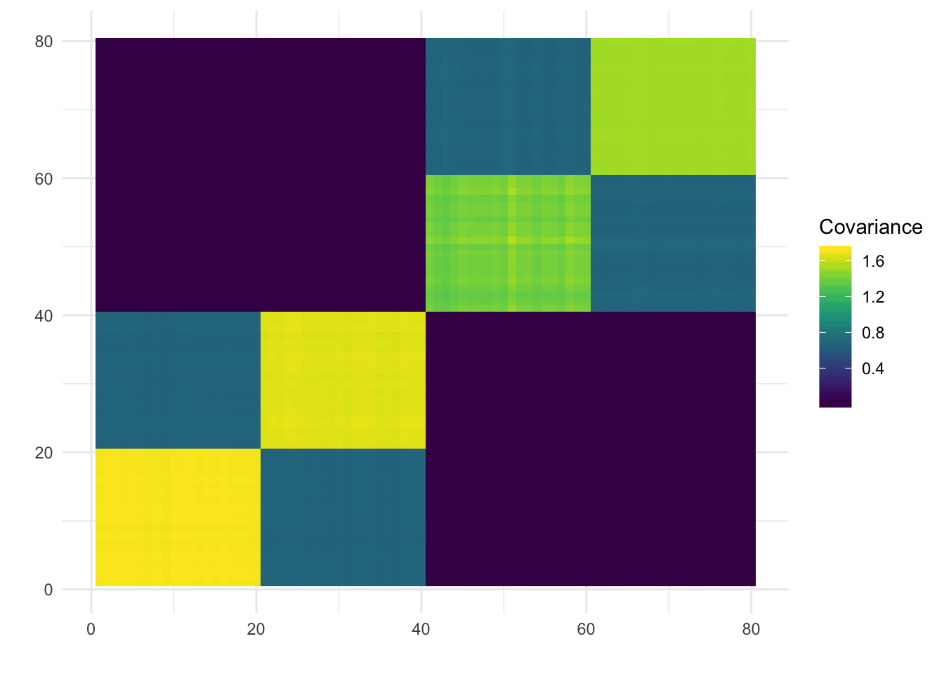
print(paste0("objective =", flash_fit_bfd$objective))[1] "objective =-716151.148219496"print(paste0("estimated residual sd =", sqrt(1 / flash_fit_bfd$fit$tau)))[1] "estimated residual sd =0.506379390822608"print("estimated prior variances (factors) =")[1] "estimated prior variances (factors) ="print(sapply(flash_fit_bfd$fit$g, function(x){1/x[[2]]$a}))[1] 1.4530330 1.4802993 0.9689280 0.4120185 0.5076058 0.6087852
sessionInfo()R version 3.5.1 (2018-07-02)
Platform: x86_64-apple-darwin13.4.0 (64-bit)
Running under: macOS 10.14.2
Matrix products: default
BLAS/LAPACK: /Users/jhmarcus/miniconda3/lib/R/lib/libRblas.dylib
locale:
[1] en_US.UTF-8/en_US.UTF-8/en_US.UTF-8/C/en_US.UTF-8/en_US.UTF-8
attached base packages:
[1] stats graphics grDevices utils datasets methods base
other attached packages:
[1] RColorBrewer_1.1-2 flashier_0.1.1 ashr_2.2-38
[4] tidyr_0.8.2 dplyr_0.8.0.1 ggplot2_3.1.0
loaded via a namespace (and not attached):
[1] Rcpp_1.0.1 compiler_3.5.1 pillar_1.3.1
[4] git2r_0.23.0 plyr_1.8.4 workflowr_1.2.0
[7] viridis_0.5.1 iterators_1.0.10 tools_3.5.1
[10] digest_0.6.18 viridisLite_0.3.0 evaluate_0.12
[13] tibble_2.0.1 gtable_0.2.0 lattice_0.20-38
[16] pkgconfig_2.0.2 rlang_0.3.1 foreach_1.4.4
[19] Matrix_1.2-15 parallel_3.5.1 yaml_2.2.0
[22] ebnm_0.1-17 xfun_0.4 gridExtra_2.3
[25] withr_2.1.2 stringr_1.4.0 knitr_1.21
[28] fs_1.2.6 rprojroot_1.3-2 grid_3.5.1
[31] tidyselect_0.2.5 glue_1.3.0 R6_2.4.0
[34] rmarkdown_1.11 mixsqp_0.1-119 reshape2_1.4.3
[37] purrr_0.3.0 magrittr_1.5 MASS_7.3-51.1
[40] codetools_0.2-16 backports_1.1.3 scales_1.0.0
[43] htmltools_0.3.6 assertthat_0.2.1 colorspace_1.4-0
[46] labeling_0.3 stringi_1.2.4 pscl_1.5.2
[49] doParallel_1.0.14 lazyeval_0.2.1 munsell_0.5.0
[52] truncnorm_1.0-8 SQUAREM_2017.10-1 crayon_1.3.4